3780
Fast 3D Undersampled Bloch-Siegert based B1+ Mapping for use in MREPT1Computer Assisted Clinical Medicine, Medical Faculty Mannheim, Heidelberg University, Mannheim, Germany, 2Electrical and Electronics Engineering, Bilkent University, Ankara, Turkey, 3Mannheim Institute for Intelligent Systems in Medicine, Medical Faculty Mannheim, Heidelberg University, Mannheim, Germany
Synopsis
Magnetic Resonance Electrical Properties Tomography (MREPT) technique utilizes complex B1+ information to obtain conductivity (σ) and permittivity (ϵ). Since obtaining B1+ magnitude is rather time consuming, several phase-based MREPT methods were previously suggested. However, these methods contain inaccuracies especially towards the periphery of the imaged object. In this paper, we utilize one of the fastest B1+ magnitude mapping techniques in order to obtain fast and accurate B1+ magnitude maps to be used in conductivity imaging. Phantom measurements show that accurate 3D B1+ magnitude maps can be acquired in less than 30 seconds, therefore improving the practicality of conductivity imaging.
Introduction
Magnetic Resonance Electrical Properties Tomography (MREPT) aims to obtain conductivity (σ) and permittivity (ϵ) which can be used for diagnostic purposes1, 2, 3. In order to obtain the electrical properties, MREPT technique requires complex (phase and magnitude) B1+ information. Although almost every pulse sequence can be used to obtain B1+ phase maps4, B1+ magnitude maps require dedicated sequences which often tend to be time consuming, especially with 3D acquisitions. Because of this issue, several methods that solely depend on B1+ phase maps were suggested5, 6, however these phase-based MREPT methods have systematic convex bias that has low-frequency nature. These errors are especially prominent towards the periphery of the imaged object since they stem from the necessary low B1+ magnitude gradient assumption4.Since B1+ magnitude is known to have spatial smoothness, there are several methods whose aim is to exploit this trait. Basically, either they utilize the concepts of parallel imaging and compress sensing7, or focus on the center of the k-space and apply various regularizations including Tikhonov8 or total generalized variation (TGV)9. Thereby, most of the information can be easily acquired in a much less acquisition time.
The purpose of this study is to investigate the utilization of TGV regularization for undersampled B1+ magnitude maps and its effect on conductivity imaging.
Methods
To acquire B1+ phase images, a 3D balanced steady-state free precession (bSSFP) pulse sequence (TE/TR = 1.5/3 ms, FoV = 256x256 mm, slice thickness = 2 mm, 32 averages, 32 slices, TA = 6:32 min:s), was used. To acquire B1+ magnitude, a GRE sequence is modified so that it has second off-resonant Fermi shaped RF pulse in accordance with Bloch-Siegert shift based B1+ mapping method. This modified 3D GRE sequence (TE/TR = 13/200 ms, FoV = 256x256 mm, slice thickness = 2 mm, 32 slices, 4 kHz off-resonance Fermi pulse, 8 ms BSS pulse duration, TA = 27:18 min:s) was used to acquire B1+ magnitude images.Fully sampled acquisitions with 128x128x32 (kx-ky-kz) k-space samples were retrospectively undersampled to 128x12x4 (Figure 1) and both were used to obtain B1+ magnitude maps through Bloch-Siegert shift based method10. For TGV regularization, which is applied to retrospectively undersampled k-space data, an open source reconstruction framework9 is used. Its underlying principle is about the minimizing the term of:
$$ \frac{\lambda}{2} \sum\limits_{j}^{N_c} ||P_+F(c_ju)-k_{j+}||^2_2 + \frac{\mu}{2} \sum\limits_{j}^{N_c} ||P_-F(c_juv)-k_{j-}||^2_2$$
where $$$\lambda$$$ and $$$\mu$$$ are regularization parameters, $$$N_c$$$ is the number of the coils, $$$P$$$ is subsampling pattern, $$$F$$$ is Fourier operator, $$$c_j$$$ is the coil sensitivity for the jth coil, $$$k_{\pm}$$$ is undersampled Fourier data corresponding to two different images ($$$I_{\pm}$$$) that are required for BSS based method, $$$I_{\pm}=|M|e^{j(\phi_0\pm\phi_{BS})}$$$, $$$\phi_{0}$$$ is the background phase, $$$\phi_{BS}$$$ is Bloch-Siegert shift, $$$u$$$ and $$$v$$$ are regularization terms that are:
$$u=|M|e^{j(\phi_0+\phi_{BS})}$$$$v\approx e^{-j2\phi_{BS}}$$
Minimizing the Eq. 1 involves two steps that utilize TGV and H1 regularization respectively:
$$\hat{u}=\frac{\lambda}{2}\sum\limits_{j}^{N_c}||P_+F(c_ju)-k_{j+}||^2_2 + TGV^2_\alpha(u)$$$$\hat{v}=\frac{\mu}{2}\sum\limits_{j}^{N_c}||P_-F(c_juv)-k_{j-}||^2_2+\frac{1}{2}||\nabla v||^2_2$$
After that, B1+ magnitude maps can be obtained via:
$$B_{1,peak}=\sqrt{\frac{-arg({\hat{v})}}{2K_{BS}}}$$
Two different techniques, namely std-MREPT11 and cr-MREPT12, were used to obtain conductivity maps from complex B1+ images. To diminish the effect of low convective field (LCF) artifact in cr-MREPT technique, data obtained from different channels in a phased-array receive coil are used together13.
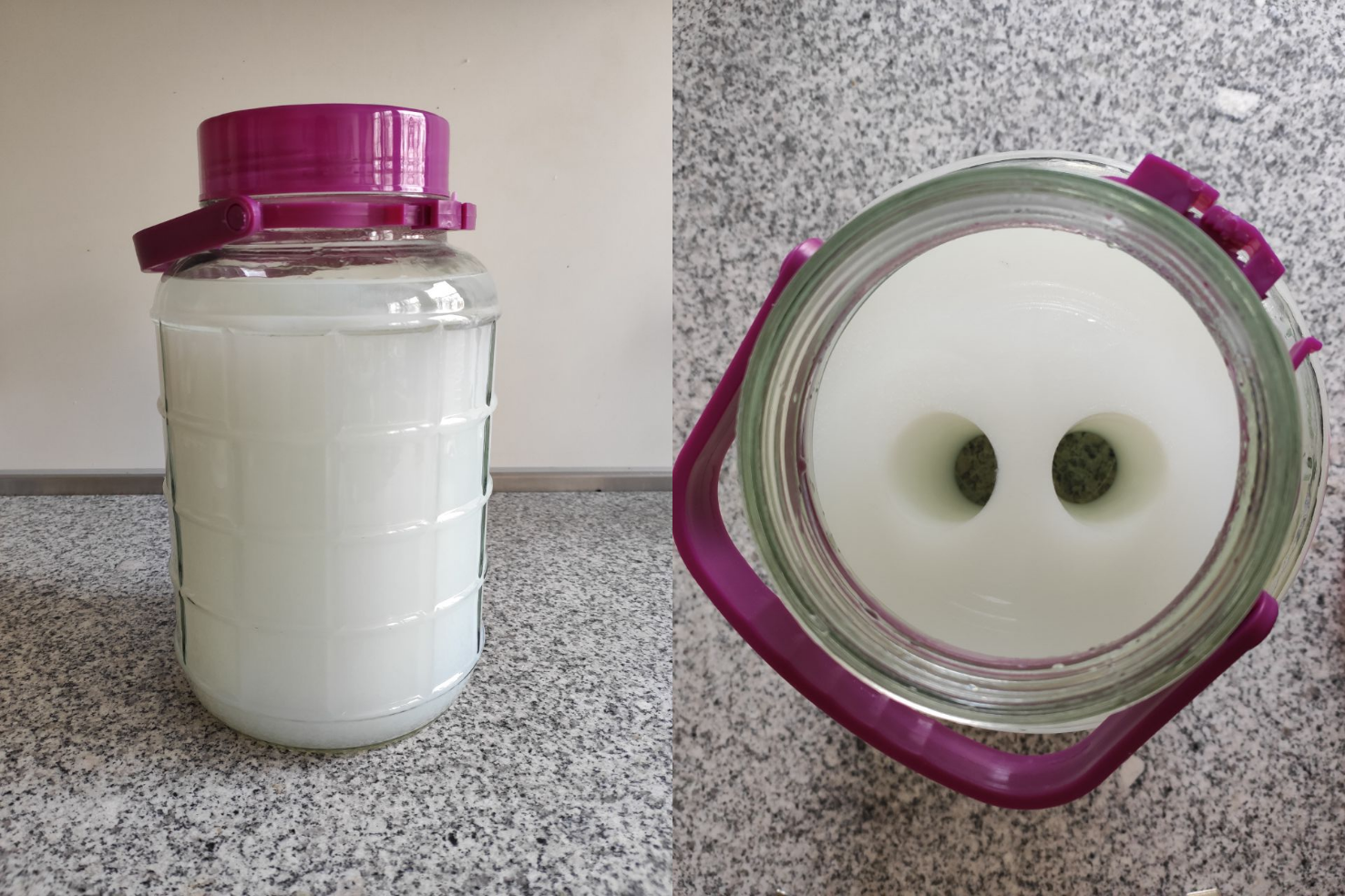
For phantom experiments, a cylindrical z-independent phantom with a diameter of 16 cm and height of 20 cm was constructed (Figure 2). For background, agar-saline solution (20 g/L agar, 2 g/L NaCl, 0.15 g/L NiCl2) was prepared and for anomalies, saline solution (6 g/L NaCl, 0.15 g/L NiCl2) was used. Anomaly regions have diameters of 3.5 cm. Experiments were conducted on 3T scanner (Magnetom Tim Trio, Siemens Healthcare GmbH, Erlangen, Germany) using a 12 channel head coil.
Results
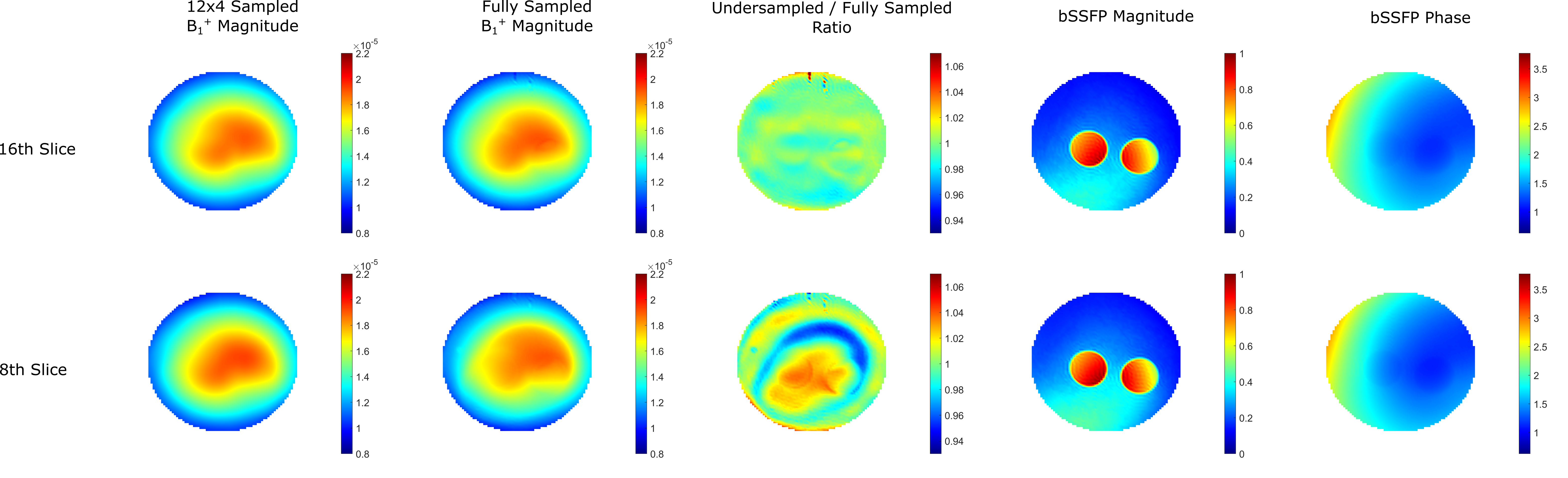
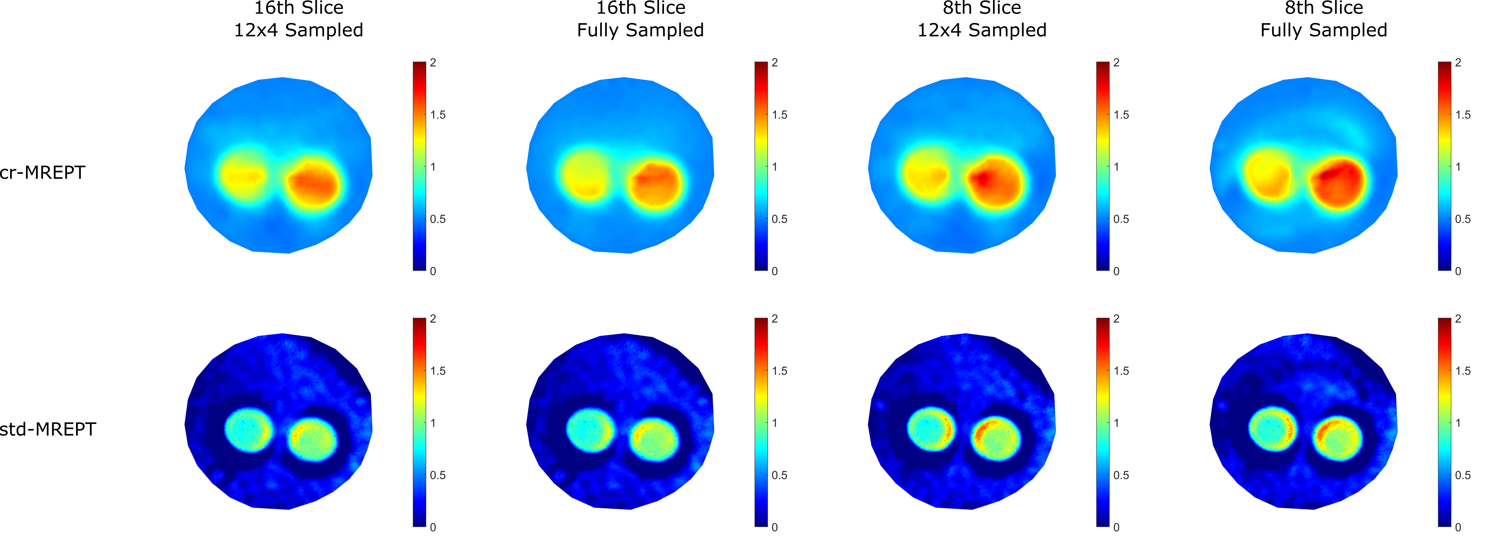
Figure 3 displays B1+ magnitude images obtained from retrospectively undersampled data (first column), fully sampled data (second column), and with their ratios (third column) for two different slices. In the 16th slice, the ratio of undersampled and fully sampled B1+ magnitudes deviates less than ±2%; however, in the 8th slice, this ratio deviates around ±5%. In addition, around the tissue boundaries, a slight deviation occurs due to missing high frequency k-space components. Figure 3 also displays bSSFP magnitude (fourth column) and phase (fifth column) images. bSSFP phase images are used as B1+ phase and bSSFP magnitude images are just given for depicting the location of the anomalies.Figure 4 shows the conductivity images that are obtained via cr-MREPT and std-MREPT techniques. It is clear that there are no visible differences between the conductivity images that are obtained from retrospectively undersampled and fully sampled B1+ magnitude images, regardless of the slice selection or choice of conductivity reconstruction technique.
Discussion and Conclusion
In this paper, we applied TGV regularization to retrospectively undersampled k-space data to obtain B1+ magnitude images. We present that there are negligible differences between fully sampled and retrospectively undersampled B1+ magnitude images. In that way, we can show that the acquisition time for obtaining B1+ magnitude can be significantly shortened (3D acquisition can be obtained in less than 30 seconds) and very accurate conductivity images can be still obtained, regardless of the slice selection or choice of conductivity reconstruction technique. All in all, reduced acquisition time can improve the practicality of conductivity imaging.Acknowledgements
No acknowledgement found.References
1. Tha, K. K., et al. "Noninvasive electrical conductivity measurement by MRI: a test of its validity and the electrical conductivity characteristics of glioma." European Radiology, vol. 28, no. 1, 2017, pp. 348-355.
2. Tha, K. K., et al. "Electrical conductivity characteristics of glioma: Noninvasive assessment by MRI and its validity." Proceedings of the 24th Annual Meeting ISMRM, Singapore, 2016; 274.
3. Gurler, N., et al. "Application of generalized phase based electrical conductivity imaging in the subacutestage of hemorrhagic and ischemic strokes." Proceedings of the 24th Annual Meeting ISMRM, Singapore, 2016; 2994.
4. Katscher, U., et al. "Recent Progress and Future Challenges in MR Electric Properties Tomography." Computational and Mathematical Methods in Medicine, vol. 2013, 2013, pp. 1-11.
5. Van Lier, A. L., et al. "B1+ Phase mapping at 7 T and its application for in vivo electrical conductivity mapping." Magnetic Resonance in Medicine, vol. 67, no. 2, 2011, pp. 552-561.
6. Gurler, N., and Ider Y.Z. "Gradient‐based electrical conductivity imaging using MR phase." Magnetic Resonance in Medicine, vol. 77, no. 1, 2016, pp. 137-150.
7. Sharma, A., et al. "Highly-accelerated Bloch-Siegert |B1+| mapping using joint autocalibrated parallel image reconstruction." Magnetic Resonance in Medicine, vol. 71, no. 4, 2013, pp. 1470-1477.
8. Zhao, F., et al. "Regularized Estimation of Magnitude and Phase of Multi-Coil B1 Field Via Bloch–Siegert B1 Mapping and Coil Combination Optimizations." IEEE Transactions on Medical Imaging, vol. 33, no. 10, 2014, pp. 2020-2030.
9. Lesch, A., et al. "Ultrafast 3D Bloch–Siegert B‐mapping using variational modeling." Magnetic Resonance in Medicine, vol. 81, no. 2, 2018, pp. 881-892.
10. Sacolick, L. I., et al. "B1 mapping by Bloch-Siegert shift." Magnetic Resonance in Medicine, vol. 63, no. 5, 2010, pp. 1315-1322.
11. Haacke, E. M., et al. "Extraction of conductivity and permittivity using magnetic resonance imaging." Physics in Medicine and Biology, vol. 36, no. 6, 1991, pp. 723-734.
12. Hafalir, F. S., et al. "Convection-Reaction Equation Based Magnetic Resonance Electrical Properties Tomography (cr-MREPT)." IEEE Transactions on Medical Imaging, vol. 33, no. 3, 2014, pp. 777-793.
13. Yildiz, G., and Ider Y.Z. "LCF Artifact Elimination in cr-MREPT using Phased-Array Receive Coil." In Proceedings of the 26th Annual Meeting of ISMRM, Paris, France, 2018; 5093.
Figures