3777
Uncertainty assessment under repeatability conditions in Helmholtz-based electric properties tomography1Istituto Nazionale di Ricerca Metrologica (INRIM), Torino, Italy, 2Philips Research Laboratories, Hamburg, Germany, 3National Physical Laboratory (NPL), Teddington, United Kingdom
Synopsis
This work shows the uncertainty evaluation under repeatability conditions of the phase-based Helmholtz-electric properties tomography (EPT) technique. Repeated MRI scans of a homogeneous cylindrical phantom are analyzed with appropriate statistical techniques to evaluate the covariance matrix of the EPT input. This matrix is propagated through the EPT technique according to the law of propagation of uncertainty. The estimated electric conductivity is highly repeatable and exhibits a spatial dispersion, whose average value, within a central region, gives an accurate estimate of the phantom conductivity. The described approach will be applied in future to extend the characterization under reproducibility conditions.
INTRODUCTION
The assessment of the uncertainty in the outcome of electric properties tomography (EPT) is of paramount importance to understand the reliability of the results and to move their interpretation from an “electric properties–weighted” to a proper quantitative imaging.The development of a complete uncertainty budget is a complex task that should be conducted according to the Guide to the expression of the uncertainty in measurement1 (GUM) and related documents,2,3 taking into account uncertainty contributions originating from different sources. The present work focuses on the repeatability contribution.
Among the EPT methods, the Helmholtz-based technique4 with phase-based approximation is here investigated due to its wider prevalence in the clinical context.5,6,7 Since this technique is a simple linear transformation from the “transceive” phase distribution $$$\varphi^\pm$$$ to the map of electric conductivity $$$\sigma$$$, the law of propagation of uncertainty1 (LPU) is applied without approximations.
METHODS
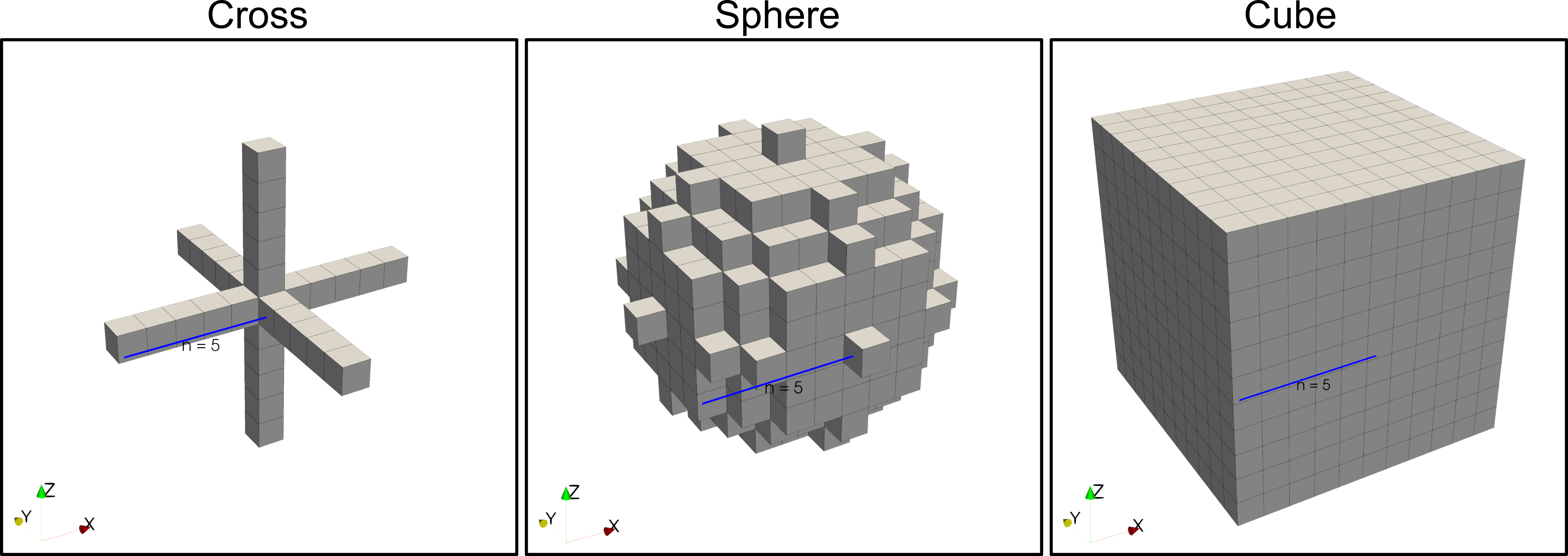
A homogeneous cylindrical phantom filled with a solution of 3.75 g/L NaCl in distilled water was scanned 25 times with an MRI scanner 3 T Ingenia TX (Philips Healthcare, Best, The Netherlands) and a 32-channel RF receive head-coil. A steady-state free precession (SSFP) sequence with low flip-angle and isotropic resolution of 2 mm was used; thus, the phase of the acquired complex images is a good approximation of $$$\varphi^\pm$$$.8 Moreover, the square root of the magnitude of the images approximates the transmit sensitivity.9 Input data were acquired in a short time and without moving the phantom, and hence under repeatability conditions. The nominal (provided with no associated uncertainty) electric conductivity of the phantom at 128 MHz is 0.56 S/m.The phase-based Helmholtz-EPT relies on the equation4,8$$\sigma=\frac{\nabla^2\varphi^\pm}{2\omega\mu_0}\,,$$whose discrete approximation can be written as $$$\boldsymbol{s}=A\boldsymbol{f}$$$, $$$\boldsymbol{f}$$$ and $$$\boldsymbol{s}$$$ being vectors describing the three-dimensional images of $$$\varphi^\pm$$$ and $$$\sigma$$$, respectively. Each row of the matrix $$$A$$$ is a local approximation, based on the Savitzky–Golay filter,10 of the differential operator $$$(2\omega\mu_0)^{-1}\nabla^2$$$, and it is characterized by the set of voxels, called kernel, used to compute it. Three kernel shapes—cross, sphere and cube—and five sizes, $$$n=1,\dots,5$$$, are investigated (Fig. 1). The EPTlib-0.1.111 implementation of Helmholtz-EPT is used.
Since the phantom is homogeneous, the spatial average $$$\overline{\sigma}$$$ of $$$\boldsymbol{s}$$$ can be taken as the phantom conductivity estimate. The generalized weighted average $$$\overline{\sigma}_w$$$, based on the covariance matrix of $$$\boldsymbol{s}$$$, $$$\Sigma(\boldsymbol{s})=A\Sigma(\boldsymbol{f})A^T$$$, is computed as well, being the minimum variance unbiased estimator of the expected value. These averages are calculated, respectively, as12$$\overline{\sigma}=N^{-1}\boldsymbol{w}^T\boldsymbol{s}\,,\quad\overline{\sigma}_w=(\boldsymbol{w}^T\Sigma(\boldsymbol{s})^{-1}\boldsymbol{w})^{-1}\boldsymbol{w}^T\Sigma(\boldsymbol{s})^{-1}\boldsymbol{s}\,,$$$$$N$$$ being the size of $$$\boldsymbol{s}$$$ and $$$\boldsymbol{w}$$$ a column vector of ones.
RESULTS
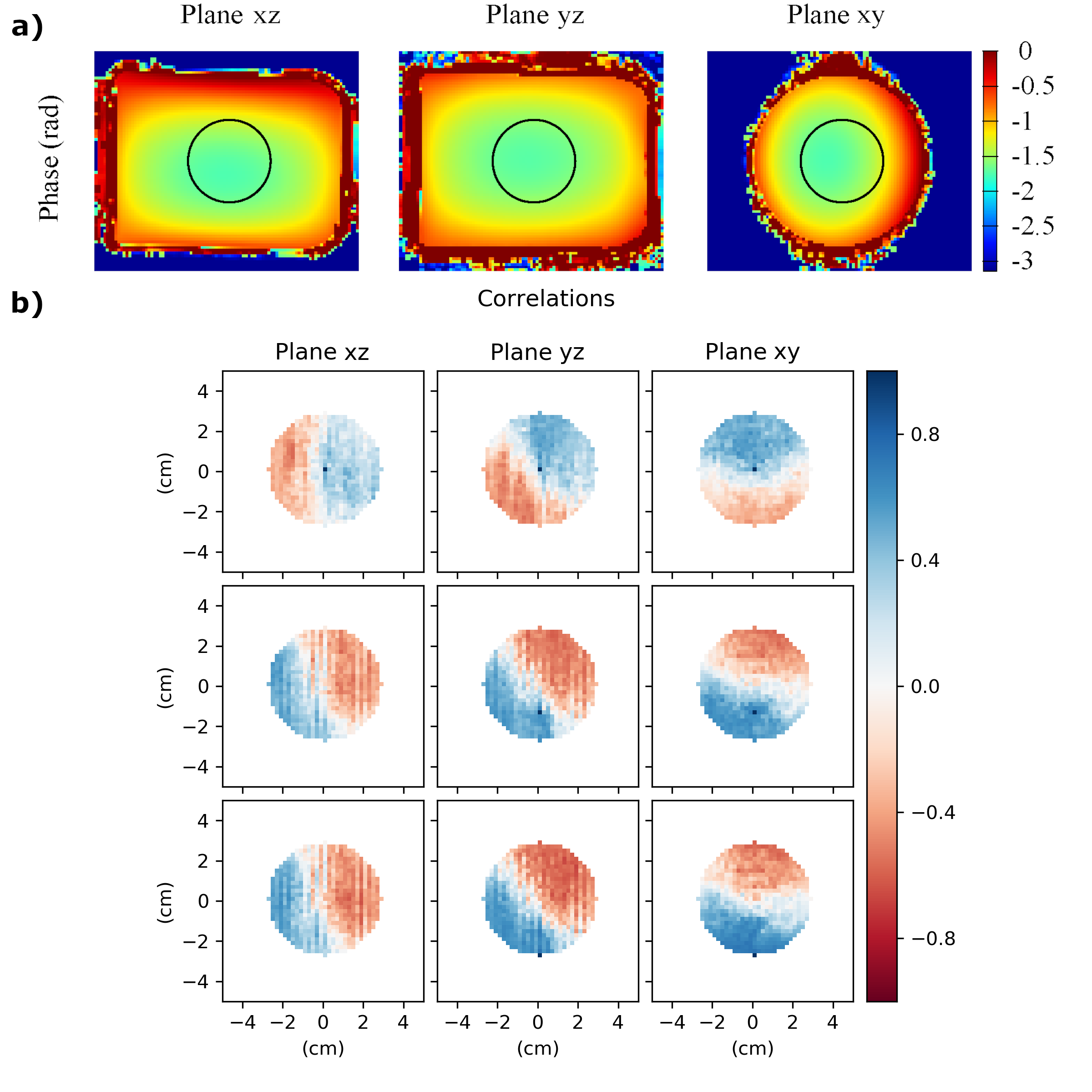
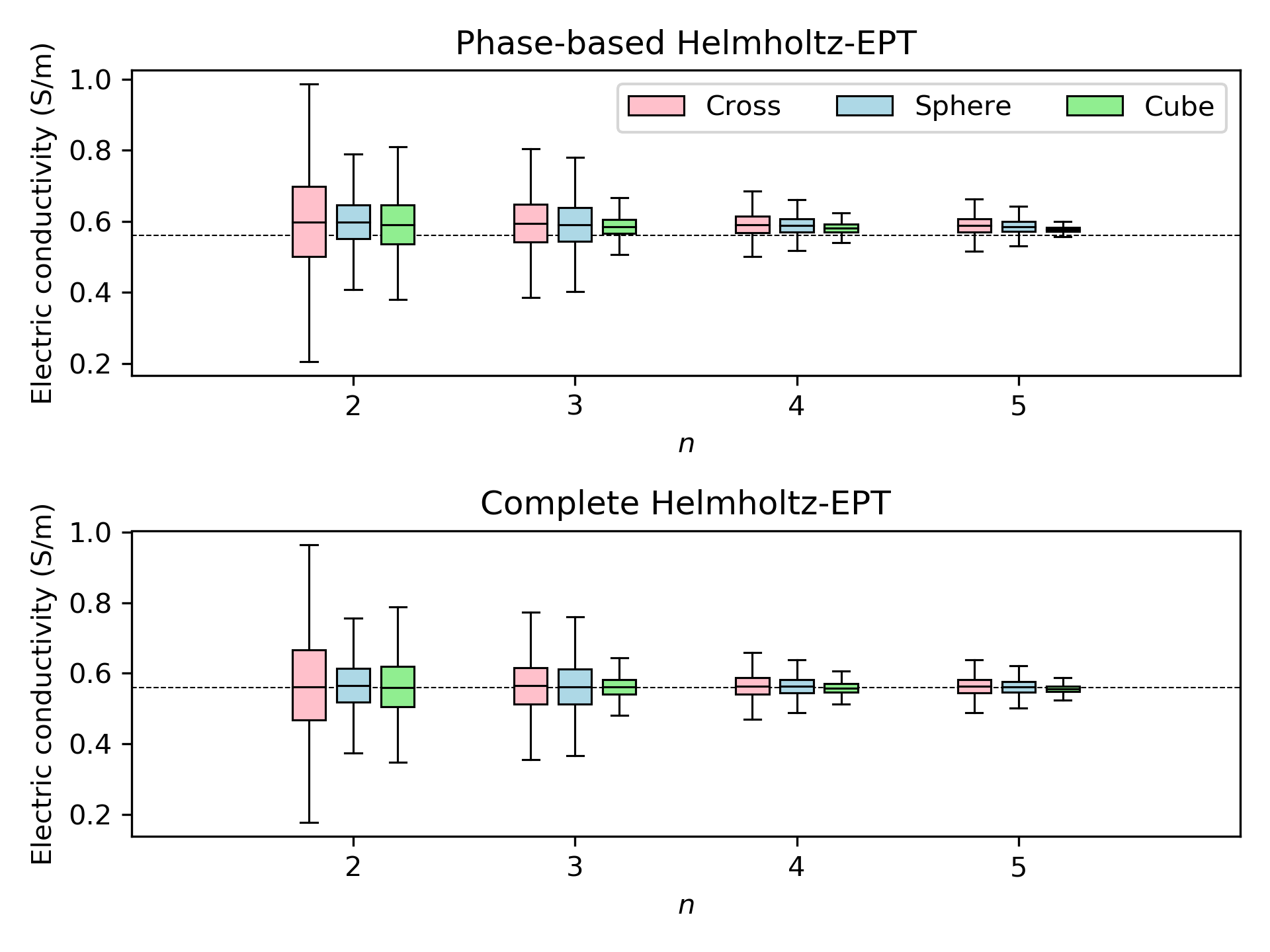
In order to reduce the dimensionality of the problem and to avoid the known issues of Helmholtz-EPT near the boundaries, only the voxels within the sphere of radius 3 cm, pictured in Fig. 2, are analyzed. Despite that, the number of voxels remains significantly larger than the number of scans; thus, to avoid the curse of dimensionality, a James–Stein-type shrinkage estimator13 for the covariance matrix $$$\Sigma(\boldsymbol{f})$$$ of the mean phase distribution $$$\boldsymbol{f}$$$ has been used. The resulting correlations are shown in Fig. 2.The conductivity map estimated by phase-based Helmholtz-EPT applied to the mean of the 25 phase distributions shows a significant spatial variability, with no regular geometrical patterns. For any kernel shape and size, the collection of $$$\boldsymbol{s}$$$ components is summarized by boxplots in Fig. 3. They show symmetric distributions whose dispersion is reduced by increasing the kernel size. Fig. 3 highlights also the systematic error due to the phase-based approximation, which is corrected by providing the magnitude of the transmit sensitivity as an additional input to Helmholtz-EPT4,8.
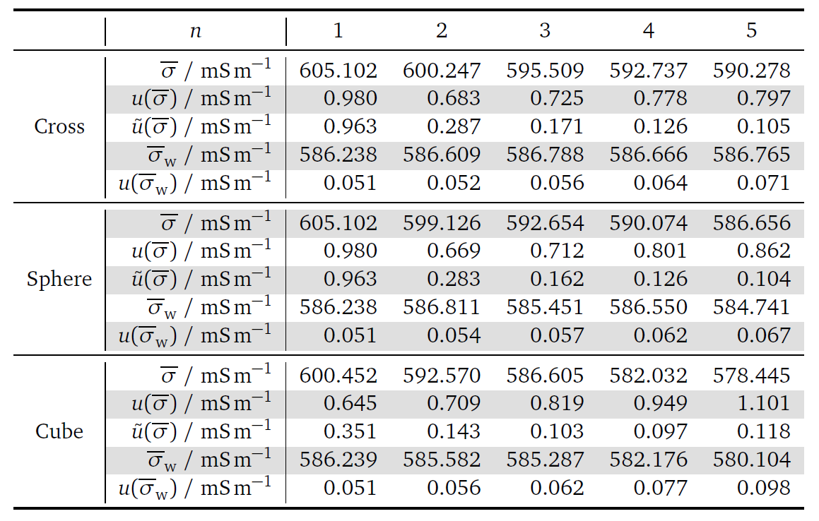
The spatial averages of the electric conductivity estimated within the sphere are collected in Fig. 4, together with their standard uncertainties12:$$u(\overline{\sigma})=N^{-1}\sqrt{\boldsymbol{w}^T\Sigma(\boldsymbol{s})\boldsymbol{w}}\,,\quad u(\overline{\sigma}_w)=\sqrt{(\boldsymbol{w}^T\Sigma(\boldsymbol{s})^{-1}\boldsymbol{w})^{-1}}\,.$$Moreover, the standard uncertainty $$$\tilde{u}(\overline{\sigma})$$$ is computed neglecting all the correlations in $$$\Sigma(\boldsymbol{f})$$$.
All data and results are available on Zenodo14.
DISCUSSION
The obtained results show that, despite a spatial dispersion of the electric conductivity estimated by phase-based Helmholtz-EPT being present under repeatability conditions, the average of the values recovered within a central sphere of voxels is a stable estimate of the nominal value of the phantom conductivity. It is weakly affected by the choice of the kernel and has a significantly small standard uncertainty, negligible with respect to the systematic error due to the phase-based approximation. The estimate is further improved, both in terms of accuracy and precision, by the generalized weighted average.The presented study suggests that the output of Helmholtz-EPT can be significantly improved by applying appropriate post-processing filters, like some kind of local averaging. In clinical investigations, for example, a median filter was adopted for cases in which the in vivo application forced the adoption of filtering volumes locally adapted to the anatomy, in order not to cross the tissue boundaries5.
CONCLUSION
A metrologically sound assessment of uncertainty in EPT has been performed under repeatability conditions with a homogeneous phantom. The obtained results show the relevance of post-processing the EPT output in order to improve the reliability. Future research will extend the proposed assessment to reproducibility conditions and heterogeneous domains.Acknowledgements
The project 17NRM05 “Examples of Measurement Uncertainty Evaluation” leading to this application has received funding from the EMPIR programme co-financed by the Participating States and from the European Union’s Horizon 2020 research and innovation programme.References
1. BIPM, IEC, IFCC, ILAC, ISO, IUPAC, IUPAP, and OIML. Guide to the Expression of Uncertainty in Measurement, JCGM 100:2008, GUM 1995 with minor corrections. BIPM, 2008.
2. BIPM, IEC, IFCC, ILAC, ISO, IUPAC, IUPAP, and OIML. Supplement 1 to the ‘Guide to the Expression of Uncertainty in Measurement’ – Propagation of distributions using a Monte Carlo method, JCGM 101:2008. BIPM, 2008.
3. BIPM, IEC, IFCC, ILAC, ISO, IUPAC, IUPAP, and OIML. Supplement 2 to the ‘Guide to the Expression of Uncertainty in Measurement’ – Extension to any number of output quantities, JCGM 102:2011. BIPM, 2011
4. Voigt T, Katscher U, and Doessel O. Quantitative conductivity and permittivity imaging of the human brain using electric properties tomography. Magn Reson Med. 2011; 66:456–466.
5. Tha KK, Katscher U, Yamaguchi S, et al. Noninvasive electrical conductivity measurement by MRI: a test of its validity and the electrical conductivity characteristics of glioma. Eur Radiol. 2018; 28:348–355.
6. Shin J, Kim MJ, Lee J, et al. Initial study on in vivo conductivity mapping of breast cancer using MRI. J Magn Reson Imaging. 2015; 42:371–378.
7. Kim S-Y, Shin J, Kim D-H, et al. Correlation between conductivity and prognostic factors in invasive breast cancer using magnetic resonance electric properties tomography (MREPT). Eur Radiol. 2016; 26:2317–2326.
8. Katscher U, Kim D-H, Seo JK. Recent progress and future challenges in MR electric properties tomography. Computational and mathematical methods in medicine. 2013; 546562.
9. Lee S-K, Bulumulla S, Wiesinger F, et al. Tissue electrical property mapping from zero echo-time magnetic resonance imaging. IEEE transactions on medical imaging. 2015; 34:541–550.
10. Savitzky A, Golay MJE. Smoothing and differentiation of data by simplified least squares procedures. Analytical chemistry. 1964; 36:1627–1639.
11. Arduino A. EPTlib 0.1.1. https://eptlib.github.io/, 2020. Accessed: 2020-09-25.
12. Cox MG, Eiø C, Mana G, Pennecchi F. The generalized weighted mean of correlated quantities. Metrologia. 2006; 43:S268–S275.
13. Schafer J, Opgen-Rhein R, Zuber V, et al. corpcor 1.6.9: Efficient Estimation of Covariance and (Partial) Correlation. http://www.strimmerlab.org/software/corpcor/, 2017. Accessed: 2020-09-29.
14. Arduino A, Pennecchi F, Zilberti L, et al. EMUE-D5-3-EPTTissueCharacterization. https://zenodo.org/communities/emue, 2020. Accessed: 2020-11-04.
Figures