Introduction

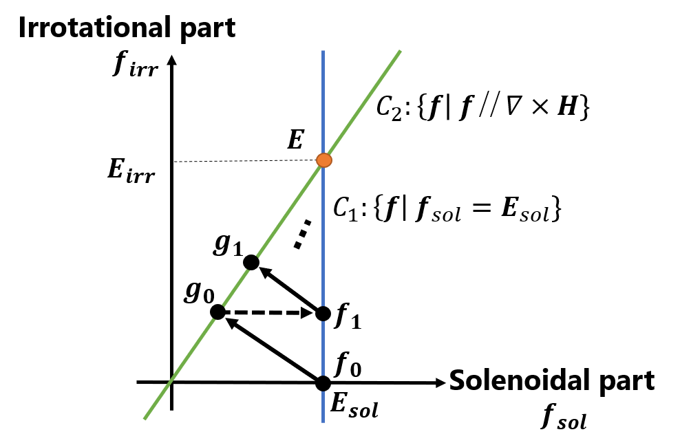
Electrical properties tomography (EPT) noninvasively estimates conductivity and permittivity distributions in the human body given a radio-frequency (RF) magnetic field ($$$H^+:=(H_x+iH_y)/2$$$)¹. The previous EPT methods accounting for spatial variations of EPs can be categorized into two types: partial-differential-equation-based (PDE-based) methods and integral-equation-based (IE-based) methods. The convection-reaction magnetic resonance electrical properties tomography (cr-MREPT) method solves the PDE for the reciprocal of admittivity, $$$1/\gamma$$$, which includes the Laplacian of $$$H^+$$$ and hence is sensitive to noise. On the other hand, the EPT methods$$$^{3,4,5,6}$$$ have been developed based on the IEs for the electromagnetic fields, which are insensitive to noise. However, convergence is not guaranteed in the iterative processes of methods$$$^{3,4}$$$ for solving the scattering problem or our previous method$$$^5$$$, which does not require a 'background' field. At ISMRM2020, we proposed a direct EPT method$$$^6$$$ for solving the IE for $$$\mathbf{E}$$$. However, the ill-posedness of the IE causes the error of EPs in this method. In this paper, we propose an IE-based method to reconstruct the electric field $$$\mathbf{E}$$$ and admittivity $$$\gamma:=\sigma+i\omega\epsilon$$$ simultaneously using the Helmholtz decomposition of $$$\mathbf{E}$$$, where $$$\sigma$$$ and $$$\epsilon$$$ are the electrical conductivity and the permittivity, respectively, and $$$\omega/2\pi$$$ is the Larmor frequency. The proposed method is shown schematically in Figure 1. We iteratively reconstruct a true electric field $$$\mathbf{E}$$$ by repeating the projections onto the vector spaces that contain the true $$$\mathbf{E}$$$. The field starts from the solenoidal part of $$$\mathbf{E}$$$, $$$\mathbf{E}_{sol}$$$, which can be computed from $$$H^+$$$ data and the boundary admittivity value. Once the algorithm converges, which is theoretically guaranteed, the true $$$\mathbf{E}$$$ and admittivity are obtained simultaneously.

Method

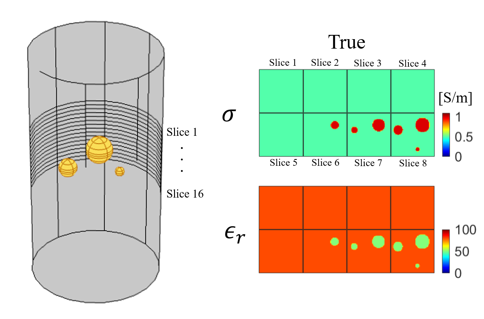
We start with the Helmholtz decomposition$$$^8$$$ of a true electric field $$$\mathbf{E}$$$ in a bounded region of interest (ROI) given by $$$\mathbf{E}=\mathbf{E}_{sol}+\mathbf{E}_{irr}$$$, where $$$\mathbf{E}_{sol}$$$ and $$$\mathbf{E}_{irr}$$$ are the solenoidal and irrotational parts of $$$\mathbf{E}$$$, respectively, which are expressed as follows⁶: \begin{align}\mathbf{E}_{sol}(\mathbf{r}')&=-\int_{\partial\Omega}({\mathbf{n}}\times\mathbf{E}(\mathbf{r}))\times\nabla\frac{1}{4\pi|\mathbf{r}-\mathbf{r}'|}\,dS+\int_{\Omega}{(\nabla\times\mathbf{E}(\mathbf{r}))\times\nabla\frac{1}{4\pi|\mathbf{r}-\mathbf{r}'|}}\,dV,\\\mathbf{E}_{irr}(\mathbf{r}')&=-\int_{\Omega}{\bigl(\mathbf{E}(\mathbf{r})\cdot\nabla\bigr)\nabla\frac{1}{4\pi|\mathbf{r}-\mathbf{r}'|}}dV.\end{align} Substituting Faraday's law, $$$\nabla\times{\mathbf{E}}=-i\omega\mu{\mathbf{H}}$$$, and Ampere's law, $$$\nabla\times\mathbf{H}=\gamma\mathbf{E}$$$, into Eq.(1) yields \begin{align}\mathbf{E}_{sol}(\mathbf{r}')&=-\int_{\partial\Omega}\biggl(\mathbf{n}\times\frac{1}{\gamma}(\nabla\times\mathbf{H})\biggr)\times\nabla\frac{1}{4\pi|\mathbf{r}-\mathbf{r}'|}\,dS-i\omega\mu\int_{\Omega}{\mathbf{H}\times\nabla\frac{1}{4\pi|\mathbf{r}-\mathbf{r}'|}}\,dV.\end{align} Assuming that $$$H_z=0$$$ and $$$|H^-|\ll|H^+|$$$ and denoting $$$\partial:=(\partial_x-i\partial_y)/2$$$, Eq.(3) is further rewritten as \begin{align}\mathbf{E}_{sol}(\mathbf{r}')&=-\int_{\partial\Omega}\biggl(\mathbf{n}\times\frac{1}{\gamma}\begin{bmatrix}-i\partial_zH^+\\ \partial_zH^+\\-4i\partial H^+\end{bmatrix}\biggr)\times\nabla\frac{1}{4\pi|\mathbf{r}-\mathbf{r}'|}\,dS-i\omega\mu\int_{\Omega}{\begin{bmatrix}H^+\\-iH^+\\0\end{bmatrix}\times\nabla\frac{1}{4\pi|\mathbf{r}-\mathbf{r}'|}}\,dV,\end{align} showing that $$$\mathbf{E}_{sol}$$$ can be computed using the measured $$$H^+$$$ and the EP values on the ROI boundary. Next, define two vector spaces \begin{align}C_1&:=\{\mathbf{f}|\mathbf{f}=\mathbf{E}_{sol}-\int_{\Omega}{\bigl(\mathbf{g}(\mathbf{r})\cdot\nabla\bigr)\nabla\frac{1}{4\pi|\mathbf{r}-\mathbf{r}'|}}dV\,\,\hbox{for any vector field}\,\,\mathbf{g}\},\\C_2&:=\{\mathbf{f}\vert\mathbf{f}\,\,\hbox{is proportional to}\,\,\nabla\times\mathbf{H}\}.\end{align} The true $$$\mathbf{E}$$$ is contained in $$$C_1$$$ for $$$\mathbf{g}=\mathbf{E}$$$ and is also contained in $$$C_2$$$ from Ampere's law $$$\mathbf{E}=\frac{1}{\gamma}\nabla\times\mathbf{H}$$$. Hence in Figure 1, the problem is to recover the true $$$\mathbf{E}$$$ as an element contained in $$$C_1\cap C_2$$$ from given $$$\mathbf{E}_{sol}$$$ (also contained in $$$C_1$$$ for $$$\mathbf{g}=\mathbf{0}$$$). For this problem we propose the use of a convex projection algorithm$$$^7$$$: starting from $$$\mathbf{E}_{sol}$$$, by repeating the orthogonal projections onto $$$C_1$$$ and $$$C_2$$$ in turn, the vector field is updated and approaches the true $$$\mathbf{E}$$$, as shown in Figure 1. To be precise, for $$$\mathbf{f}_n\in C_1$$$ at step $$$n$$$, its projection onto $$$C_2$$$ is given by \begin{align}\mathbf{g}_n&=\Bigl(\frac{\mathbf{f}_n\cdot(\nabla\times\mathbf{H})^*}{|\nabla\times\mathbf{H}|^2}\Bigr)\nabla\times\mathbf{H}.\end{align} Then, for $$$\mathbf{g}_n\in C_2$$$, its projection onto $$$C_1$$$ is given by \begin{align}\mathbf{f}_{n+1}&=\mathbf{E}_{sol}-\int_{\Omega}{\bigl(\mathbf{g}_n\cdot\nabla\bigr)\nabla\frac{1}{4\pi|\mathbf{r}-\mathbf{r}'|}}dV.\end{align} Setting the initial field as $$$\mathbf{f}_0:=\mathbf{E}_{sol}$$$, we update the vector fields using Eqs.(7) and (8) iteratively. The convergence of the algorithm is theoretically guaranteed because $$$C_1$$$ and $$$C_2$$$ are convex sets$$$^7$$$. It is remarkable that when the algorithm converges to obtain $$$\mathbf{f}_{\infty}=\mathbf{E}$$$, it holds that $$$\frac{\mathbf{f}_\infty\cdot(\nabla\times\mathbf{H})^*}{|\nabla\times\mathbf{H}|^2}=\frac{\mathbf{E}\cdot(\nabla\times\mathbf{H})^*}{|\nabla\times\mathbf{H}|^2}=\frac{1}{\gamma}$$$ from Ampere's law. Therefore, when $$$\mathbf{E}$$$ is estimated, $$$\gamma$$$ can be automatically determined.

We verified our method through numerical simulations. In the simulations, the $$$H^+$$$ data was computed using FEM software (COMSOL Multiphysics, COMSOL Inc.). The following two situations were modeled: Model 1 was a simple model including three spheres with higher conductivity ($$$\sigma=1.0$$$ S/m) and lower relative permittivity ($$$\epsilon_r=50$$$) as compared to the background material ($$$\sigma=0.5$$$ S/m, $$$\epsilon_r=80$$$), as shown in Figure 2. Model 2 is a head model$$$^9$$$. We compared the proposed method with our previous direct method$$$^6$$$.

Results & Discussion

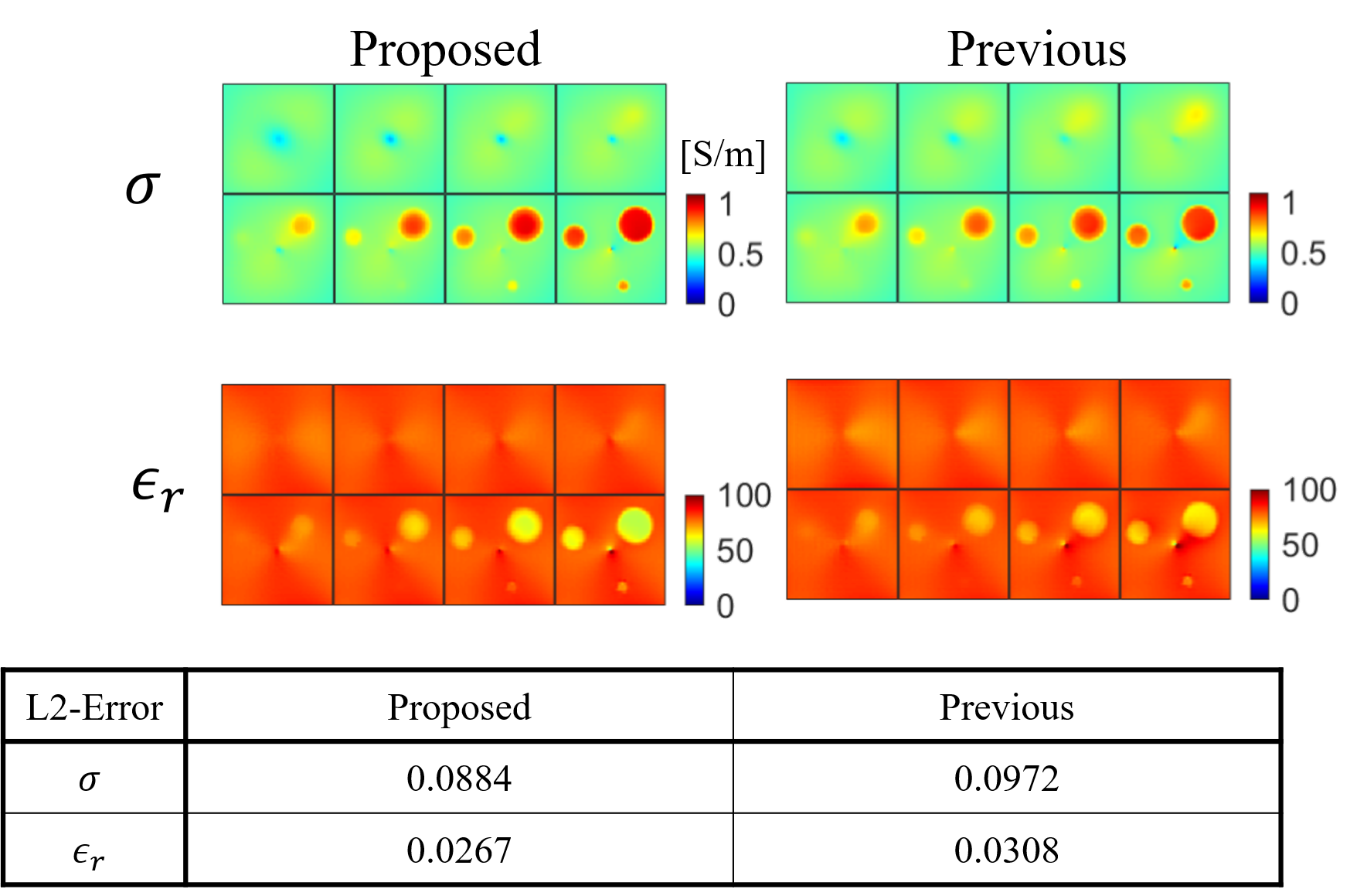
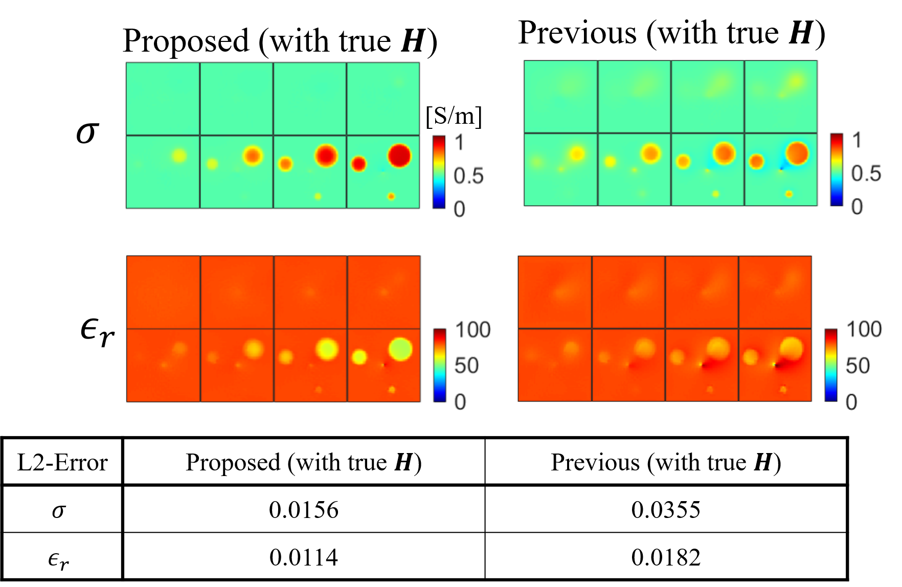
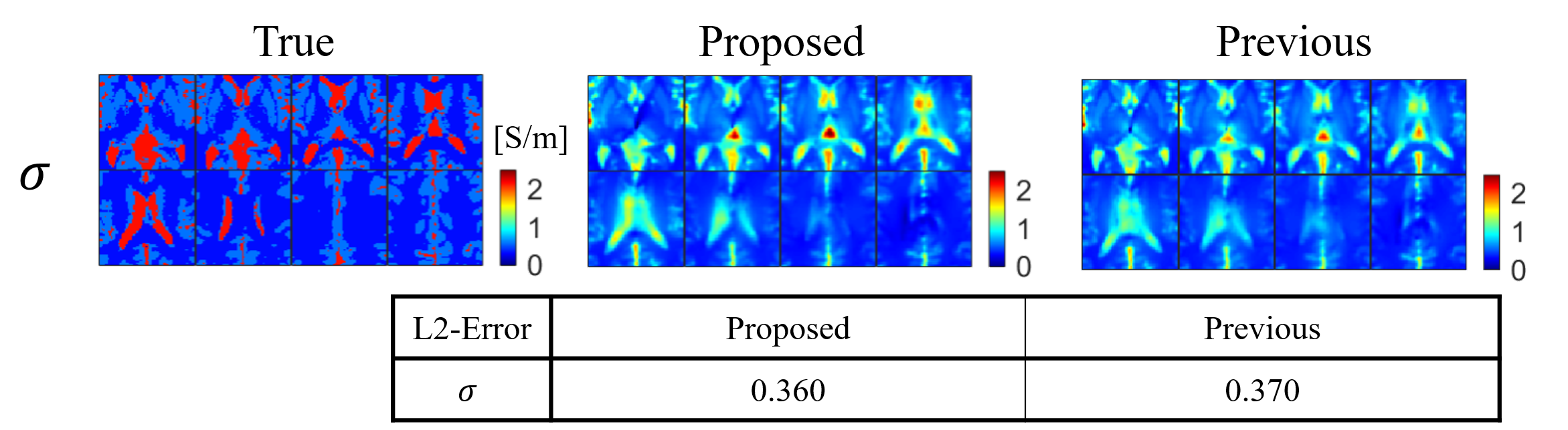
The proposed method outperformed the previous method with Model 1 and Model 2 (Figure 3 and Figure 5). This may be due to the improvement of the ill-posedness of the previous method by adding the constraint that $$$\mathbf{E}$$$ is proportional to $$$\nabla\times\mathbf{H}$$$ in the proposed method. Thus, in the proposed method, the errors of EPs may be only caused by the approximation of $$$\mathbf{H}$$$ by $$$H^+$$$. The proposed method can reconstruct true EP maps using Eq.(3) with the true $$$\mathbf{H}$$$ of Model 1, whereas the previous method cannot due to the ill-posedness (Figure 4). It is observed that artifacts around the center are reduced if $$$\mathbf{H}$$$ can be used. The difference between the proposed method and the method proposed by us (#1434) is whether the formulation includes $$$H^+$$$ only or $$$\mathbf{H}$$$. In contrast to the method (#1434), the method in this paper has a characteristic that it is formulated using $$$\mathbf{H}$$$ and hence has the potential to reduce the artifact if components of $$$\mathbf{H}$$$ other than $$$H^+$$$ such as $$$H^-$$$ can be incorporated. Combining the method$$$^{10}$$$ to compute $$$H^-$$$ with the proposed method will be an important aspect in future studies.

Conclusion

In this paper, we proposed a novel, IE-based EPT method using the Helmholtz decomposition, which was verified numerically. If all of the components of $$$\mathbf{H}$$$ are available, the proposed method has the potential to suppress artifacts, which is the problem in the conventional methods.

Acknowledgements

The present study was financially supported by Canon Medical Systems Corporation.