3775
Optimal Kernel Radii for Calculating the Derivatives of Noisy B1 Phase for Accurate Phase-Based Quantitative Conductivity Mapping1Department of Medical Physics and Biomedical Engineering, University College London, London, United Kingdom
Synopsis
Quantitative conductivity mapping (QCM) techniques use the first spatial derivatives and/or the Laplacian of the B1 phase. These are commonly estimated by fitting a 3D quadratic function within a kernel around each voxel. However, small kernels lead to severe noise amplification and large kernels induce inaccuracies. Here we determined the optimal kernel radii across a range of magnitude SNR using an anthropomorphic, numerical brain phantom. The optimal kernel size decreased with increasing SNR. Calculating the first derivatives required smaller kernels than calculating the Laplacian making QCM methods using first derivatives likely more accurate than Laplacian-based techniques.
Purpose
MR Electrical Properties Tomography (EPT) is a novel, non-invasive technique that calculates tissue permittivity and electrical conductivity from the complex B1 field1. Tissue conductivity ($$$\sigma$$$), often calculated from the B1 phase ($$$\varphi_0$$$), may provide new information on tissue ion content, specifically on sodium levels2, and quantitative conductivity mapping (QCM) shows promise for distinguishing between tumour types e.g. in the brain3.Almost all QCM techniques require calculation of the first spatial derivatives, $$$(\partial_x,\partial _y,\partial_z)$$$, and/or the Laplacian, $$$\nabla^2=(\partial_x^2+\partial_y^2+\partial_z^2)$$$, of $$$\varphi_0$$$1,4,5. However, using finite difference approximation tends to severely amplify the noise6,7. One widely-used noise suppression method involves locally fitting a 3D quadratic function to $$$\varphi_0$$$ within a kernel around each voxel and calculating the derivatives of the fitted function8-10. This idea is motivated by the fact that in regions with slowly varying $$$\sigma$$$:
$$\sigma=(\mu_0\omega)^{-1}\cdot\nabla^2\varphi_0\quad[1]$$
$$$\mu_0$$$=vacuum permeability and $$$\omega$$$=Larmor angular frequency. In 1D, $$$\varphi_0$$$ is restricted to be quadratic in regions of homogeneous $$$\sigma$$$ where $$$\nabla^2\varphi_0$$$ is also homogenous (Equation 1).
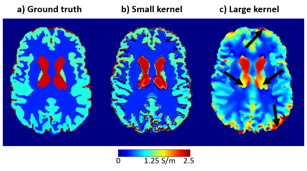
However, in 3D, there are an infinite number of possible higher-order terms in $$$\varphi_0$$$ with zero Laplacian, e.g. $$$\nabla^2(x^3-3xy^2)=0$$$. Therefore, 3D quadratic fitting results in inaccurate derivatives even in a noise-free phantom (Figure 1), especially when using large kernels where higher-order terms have a greater effect. This suggests that an optimal kernel radius represents a balance between noise suppression and accuracy. Here, we determine the optimal kernel radii for calculating the first derivatives and the Laplacian of $$$\varphi_0$$$ for a range of noise levels using an anthropomorphic, numerical brain phantom.
Methods
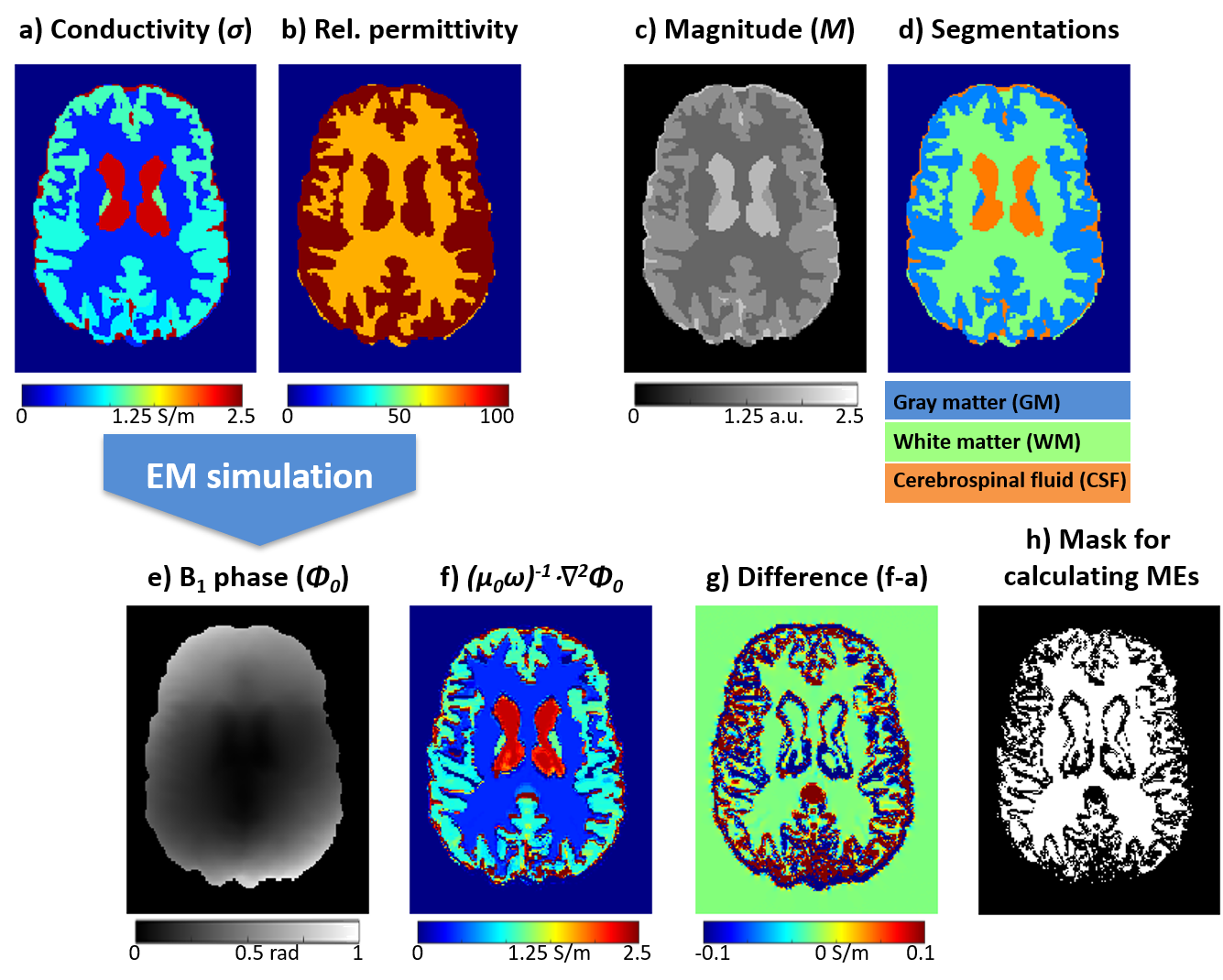
Realistic conductivity11, permittivity11, and (gradient-echo) magnitude ($$$M$$$) images (Figure 2) were generated using a version of the Zubal brain phantom12,13 upsampled to 1 mm isotropic resolution. The noise-free B1 phase, $$$\phi_0$$$, was calculated from the phantom conductivity and permittivity using established 3D electromagnetic simulations14-16. The incident electric field was defined as the field generated by an infinitely long, 16-rung, 60-cm-diameter quadrature birdcage coil.Noisy magnitude, $$$m$$$, and $$$\varphi_0$$$ were simulated by adding Gaussian noise (14 different magnitude signal-to-noise ratio (SNR) = 5 to 105) to the real and imaginary components of the complex signal, $$$M\cdot\exp(i\phi_0)$$$. A range of kernel radii (1–20 mm, step size=1 mm) were used to calculate the first derivatives and the Laplacian of the noisy $$$\varphi_0$$$ and only the smallest kernel was used to calculate the noise-free derivatives from $$$\phi_0$$$. To avoid blurring and inaccuracies near the tissue boundaries where Equation 1 is not applicable, it is common practice to restrict these kernels to segmented regions17 that are expected to have homogeneous conductivities (Figure 2d). The SNR was calculated as the ratio of the mean and standard deviation of m within the white matter, while the mean absolute errors (ME) in the first derivatives and Laplacian were computed as follows:
$$ME_i = mean(|\partial_i\varphi_0-\partial_i\phi_0|)\,for\,i=x,y,z\quad[2]$$
$$ME_1 = (ME_x+ME_y+ME_z)/3\quad[3]$$
$$ME_2 = mean(|(\partial_x^2+\partial_y^2+\partial_z^2)\varphi_0-(\partial_x^2+\partial_y^2+\partial_z^2)\phi_0|)\quad[4]$$
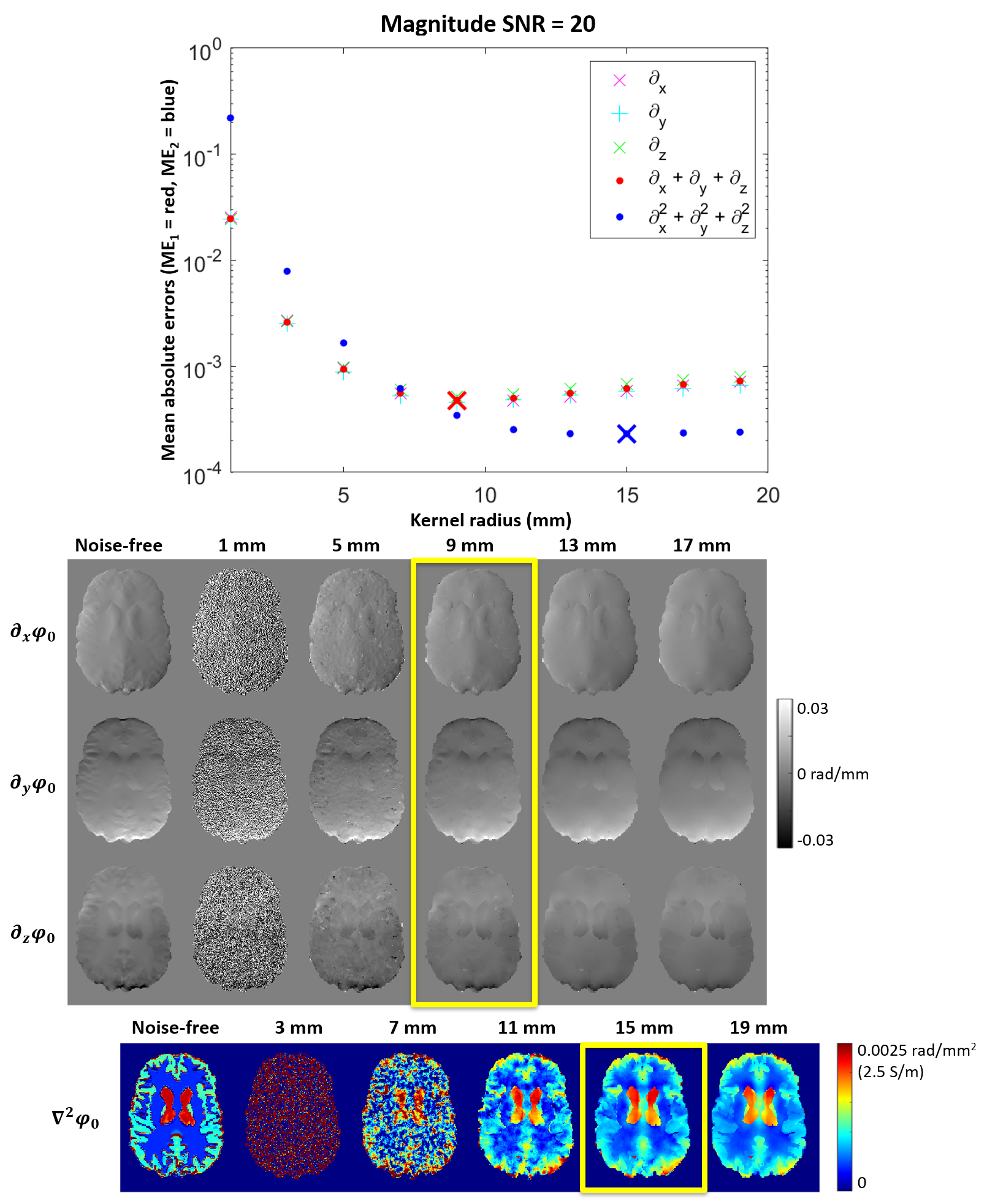
For all $$$ME$$$, the mean was calculated throughout the brain excluding the conductivity boundaries, where $$$\sigma\neq(\mu_0\omega)^{-1}\cdot\nabla^2\phi_0$$$, (Figure 2f-h). At each SNR, the kernel radii corresponding to the minimum error in the first spatial derivatives ($$$ME_1$$$) and the Laplacian ($$$ME_2$$$) were selected as optimal (Figure 3). Instead of determining individual optimised kernel radii for the first derivatives in the x, y, and z directions (based on $$$ME_{x/y/z}$$$), we used the mean of the individual errors ($$$ME_1$$$) to select a unified, optimal kernel size as spatial derivatives in all three directions are required for QCM and using three different kernels would triple the processing time for calculating the derivatives. In any case, $$$ME_{x/y/z}$$$ and $$$ME_1$$$ (and corresponding kernel sizes) were almost identical (Figure 3, top).
Results
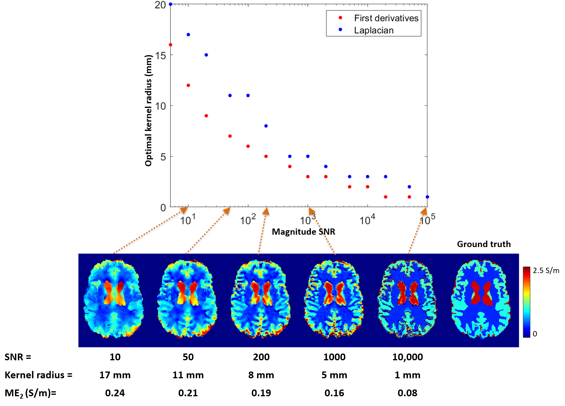
Figure 3 shows $$$ME_1$$$ and $$$ME_2$$$ plotted as a function of the kernel radius at SNR=20 and example derivative maps. Note that the scaled Laplacian of the noise-free phase $$$(\mu_0\omega)^{-1}\cdot\nabla^2\phi_0$$$ (Figure 3 bottom left) represents an accurate reconstruction of the original conductivity map (Figure 2a) within homogeneous regions, as expected from Equation 1. The minimum-error kernel radii gave derivative maps most visually similar to the noise-free maps (Figure 3, yellow rectangles). The optimal kernel radii represent a trade-off between noise suppression (larger radii) and accuracy (smaller radii, Figure 1).Figure 4 shows the optimal kernel radii for calculating the first derivatives and the Laplacian of $$$\varphi_0$$$ as a function of SNR. As expected, higher SNR allows for smaller kernels and low SNR requires larger ones. For each SNR, the first derivatives can be accurately calculated with a smaller kernel than the Laplacian. In vivo, conductivity distributions are expected to vary even within tissue types (i.e. gray matter or white matter). Since Equation 1 is only applicable within regions of homogeneous conductivity, smaller optimal kernels are anticipated to lead to more accurate results making QCM methods that use only the first derivatives of $$$\varphi_0$$$ likely more accurate than Laplacian-based techniques.
Conclusions
We determined optimal kernel radii for calculating the first derivatives and the Laplacian of the B1 phase for a range of SNR. Calculating the first derivatives required smaller kernels than calculating the Laplacian, conferring an advantage on first-derivative-based QCM techniques.Acknowledgements
Dr Anita Karsa, Dr Patrick Fuchs, and Dr Karin Shmueli were supported by European Research Council Consolidator Grant DiSCo MRI SFN 770939.References
1. Katscher, Ulrich, and Cornelius AT van den Berg. "Electric properties tomography: biochemical, physical and technical background, evaluation and clinical applications." NMR in Biomedicine 30.8 (2017): e3729.
2. Liao, Yupeng, et al. "Correlation of quantitative conductivity mapping and total tissue sodium concentration at 3T/4T." Magnetic resonance in medicine 82.4 (2019): 1518-1526.
3. Tha, Khin Khin, et al. "Noninvasive electrical conductivity measurement by MRI: a test of its validity and the electrical conductivity characteristics of glioma." European radiology 28.1 (2018): 348-355.
4. Katscher, Ulrich, Dong-Hyun Kim, and Jin Keun Seo. "Recent progress and future challenges in MR electric properties tomography." Computational and mathematical methods in medicine 2013 (2013).
5. Gurler, Necip, and Yusuf Ziya Ider. "Gradient‐based electrical conductivity imaging using MR phase." Magnetic resonance in medicine 77.1 (2017): 137-150.
6. Mandija, Stefano, et al. "Error analysis of helmholtz‐based MR‐electrical properties tomography." Magnetic resonance in medicine 80.1 (2018): 90-100.
7. Karsa, Anita, and Shmueli, Karin. “Simultaneous Noise Suppression and Edge Preservation in Phase-based MRI Conductivity Mapping.” Proceedings of the Annual Meeting of the ESMRMB. (2020).
8. Voigt, Tobias, Ulrich Katscher, and Olaf Doessel. "Quantitative conductivity and permittivity imaging of the human brain using electric properties tomography." Magnetic Resonance in Medicine 66.2 (2011): 456-466.
9. Van Lier, Astrid LHMW, et al. "B1 phase mapping at 7 T and its application for in vivo electrical conductivity mapping." Magnetic Resonance in Medicine 67.2 (2012): 552-561.
10. Lee, Joonsung, Jaewook Shin, and Dong‐Hyun Kim. "MR‐based conductivity imaging using multiple receiver coils." Magnetic resonance in medicine 76.2 (2016): 530-539.
11. Voigt, Tobias, Ulrich Katscher, and Olaf Doessel. "Quantitative conductivity and permittivity imaging of the human brain using electric properties tomography." Magnetic Resonance in Medicine 66.2 (2011): 456-466.
12. Zubal, I. George, et al. "Two dedicated software, voxel-based, anthropomorphic (torso and head) phantoms." Proceeding of the International Conference at the National Radiological Protection Board. 1995.
13. Karsa, Anita, Shonit Punwani, and Karin Shmueli. "The effect of low resolution and coverage on the accuracy of susceptibility mapping." Magnetic resonance in medicine 81.3 (2019): 1833-1848.
14. Remis, Rob, and Edoardo Charbon. "An electric field volume integral equation approach to simulate surface plasmon polaritons." Advanced Electromagnetics 2.1 (2013): 15-24.
15. Chew, Weng Cho, Mei Song Tong, and Bin Hu. "Integral equation methods for electromagnetic and elastic waves." Synthesis Lectures on Computational Electromagnetics 3.1 (2008): 1-241.
16. Leijsen, Reijer, et al. "Developments in electrical-property tomography based on the contrast-source inversion method." Journal of Imaging 5.2 (2019): 25.
17. Katscher, Ulrich, et al. "Estimation of breast tumor conductivity using parabolic phase fitting." Proceedings of the 20th Annual Meeting of the ISMRM. (2012): 3482.
Figures