3774

New Approaches for Simultaneous Noise Suppression and Edge Preservation to Achieve Accurate Quantitative Conductivity Mapping in Noisy Images

Anita Karsa¹ and Karin Shmueli¹
¹Department of Medical Physics and Biomedical Engineering, University College London, London, United Kingdom

Synopsis

Due to their extreme noise amplification, current Quantitative Conductivity Mapping (QCM) techniques require high SNR images. Simultaneous Quantitative Susceptibility Mapping and QCM uses low-SNR gradient-echo sequences, creating a need for QCM methods appropriate for noisy images. Here we proposed, optimised, and compared several new QCM methods (all shared on https://xip.uclb.com/i/software/MRI_conductivity.html) built on the widely-used phase-based formula and its equivalent, less popular integral form. We found that solving the integral equation provided lower errors and better edge preservation in both simulated and in-vivo images, and that edge preservation combining magnitude-based and image-segmentation-based techniques resulted in the best in-vivo conductivity map.

Purpose

Quantitative Conductivity Mapping (QCM) is a non-invasive technique that calculates the tissue electrical conductivity from the B₁ phase ($$$\varphi_0$$$)¹. Tissue conductivity ($$$\sigma$$$) may provide new information on sodium levels², and can distinguish between different types of brain glioma³.

In state-of-the-art QCM, $$$\varphi_0$$$ is usually acquired using high signal-to-noise ratio (SNR) sequences^1,4,5, but some studies^6-8 have begun to apply simultaneous Quantitative Susceptibility Mapping (QSM) and QCM using gradient-echo (GRE) imaging. To compensate for the low SNR of GRE, these studies use Gaussian filtering, reducing the apparent resolution. Here we propose, optimise, and compare new QCM methods for low-SNR data to expand the applicability of QCM to low-SNR sequences and facilitate further studies into simultaneous QSM/QCM.

Theory

The following differential equation is a widely-used approximation¹, valid in regions with slowly varying $$$\sigma$$$:
$$\sigma=(\mu_0\omega)^{-1}\cdot\nabla^2\varphi_0\quad[1]$$
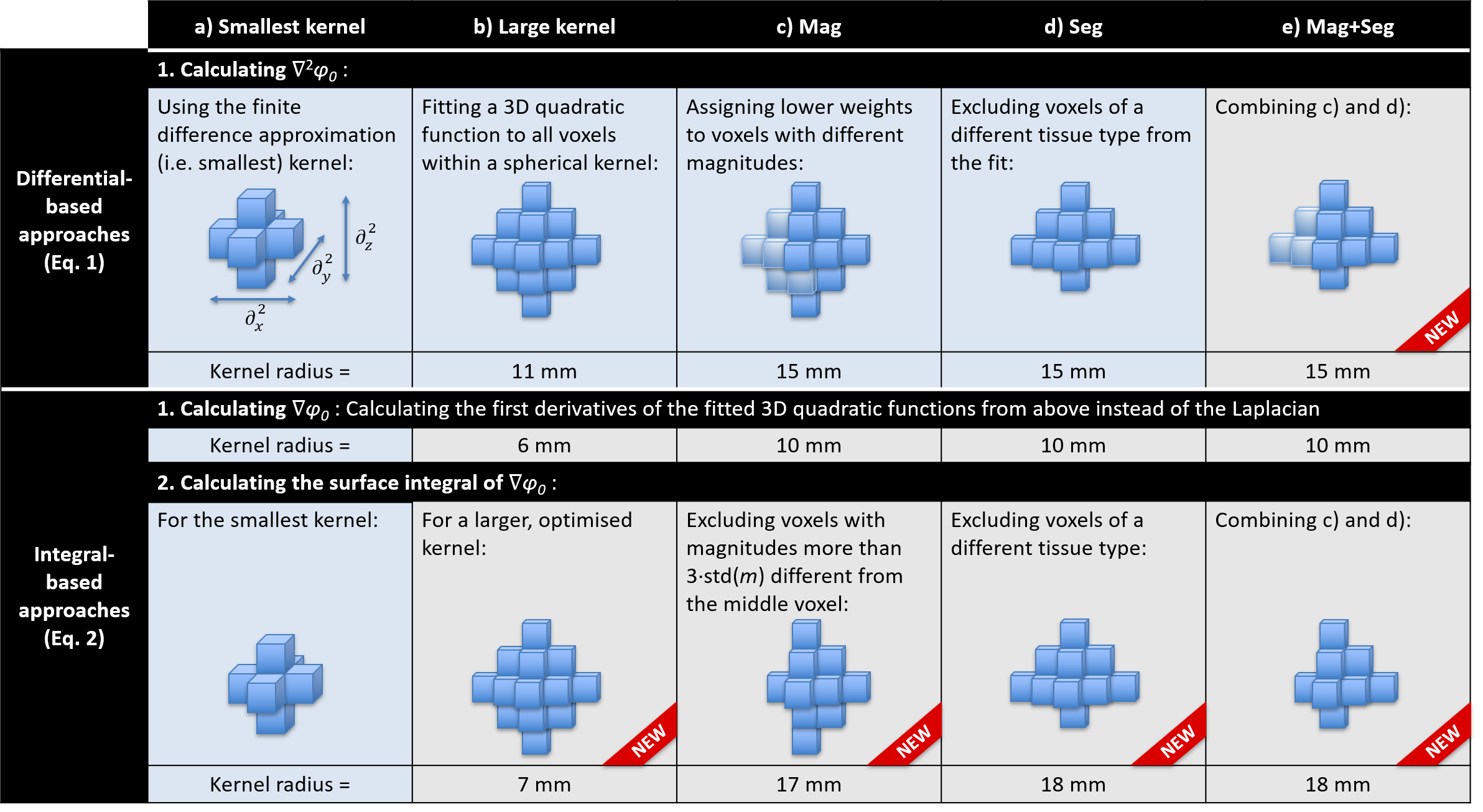
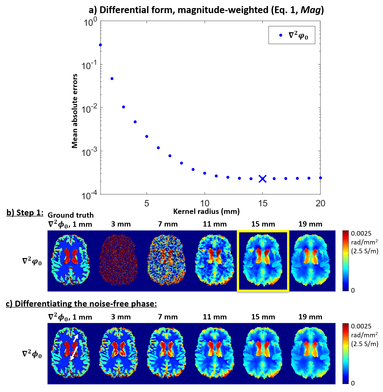
$$$\mu_0=$$$vacuum permeability, $$$\omega=$$$Larmor frequency, and $$$\nabla^2=$$$Laplacian operator. Applying a finite-difference approximation of $$$\nabla^2$$$ (Figure 1a) severely amplifies the noise⁹, especially in low-SNR data (Figure 5a). One widely-used noise suppression method involves fitting a 3D quadratic function within a kernel around each voxel and calculating the Laplacian of these fitted functions^5,10 (Figure 1b). However, this results in blurring near the conductivity boundaries (Figure 5b) where Equation 1 is not applicable.

It has been suggested previously that the integral form¹¹ of Equation 1 is more noise robust¹²:
$$\sigma=(V\mu_0\omega)^{-1}\cdot\int_S\nabla\varphi_0d\textbf{s}\quad[2]$$
where $$$S$$$ is the closed surface of some kernel with volume $$$V$$$.

Previous studies have used i) Equation 1 with large kernels combined with either magnitude-based weighting⁵ (Mag) (Figure 1c) or magnitude-based image segmentation¹³ (Seg) (Figure 1d) for better edge preservation, or ii) Equation 2 only with small kernels to avoid errors at the conductivity boundaries^11-12 (Figure 1a).

Here we implemented Equations 1 and 2 using large kernels restricted by the magnitude (Mag) and/or the segmentation (Seg) (Figure 1b-e).

Methods

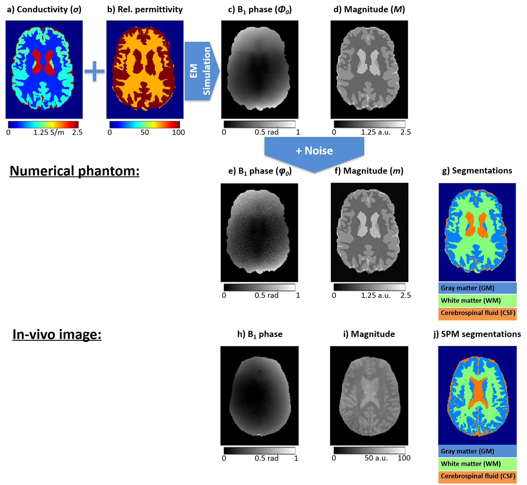
Multi-echo GRE brain images (Figure 2, bottom) were acquired in a healthy volunteer at 3T¹⁴ (Prisma, Siemens) using a 64-channel RF coil with FOV=22×22×13 cm³, 1.5 mm isotropic resolution, TR=4370 ms, and α=90°. ASPIRE¹⁵ was used on the first two echoes (TE₁=5 ms and TE₂=10 ms) to estimate $$$\varphi_0$$$ (the phase at TE=0 ms) for each channel which were then combined using scalar phase matching¹⁶. Gray matter (GM), white matter (WM), and the cerebrospinal fluid (CSF) were segmented using SPM12¹⁷ on the combined magnitude image at TE=0 ms (extrapolated using an exponential fit followed by bias field correction¹⁸). The SNR was calculated as the ratio of the extrapolated $$$M_0$$$ mean and standard deviation within WM.

Realistic conductivity¹¹, permittivity¹¹, and signal magnitude ($$$M$$$) values were assigned to an anthropomorphic numerical brain phantom^19,20 with 1 mm isotropic resolution (Figure 2, top). The noise-free B₁ phase, $$$\phi_0$$$, was calculated from the phantom conductivity and permittivity maps using established 3D electromagnetic simulations^21-23. The incident electric field was defined as the field generated by an infinitely long, 16-rung, 60-cm-diameter, quadrature birdcage coil. Noisy magnitude, $$$m$$$, and $$$\varphi_0$$$ were simulated by adding Gaussian noise to the real and imaginary components of the complex signal, $$$M\cdot\exp(i\phi_0)$$$ matching the SNR (=16) of the phantom to the in-vivo image.

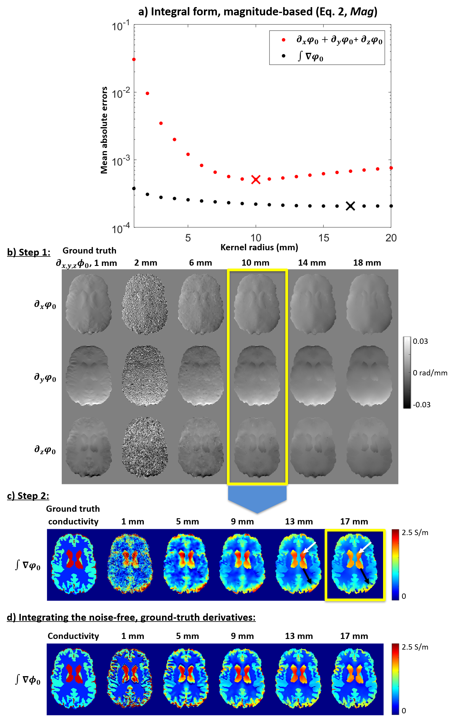
Conductivity maps were calculated from the in-vivo and simulated $$$\varphi_0$$$ using all 10 methods in Figure 1 and optimal kernel radii determined by finding the minimum mean absolute error throughout the numerical brain phantom (Figures 3a-b and 4a-c) where true derivatives were calculated from the noise-free $$$\phi_0$$$.

Results

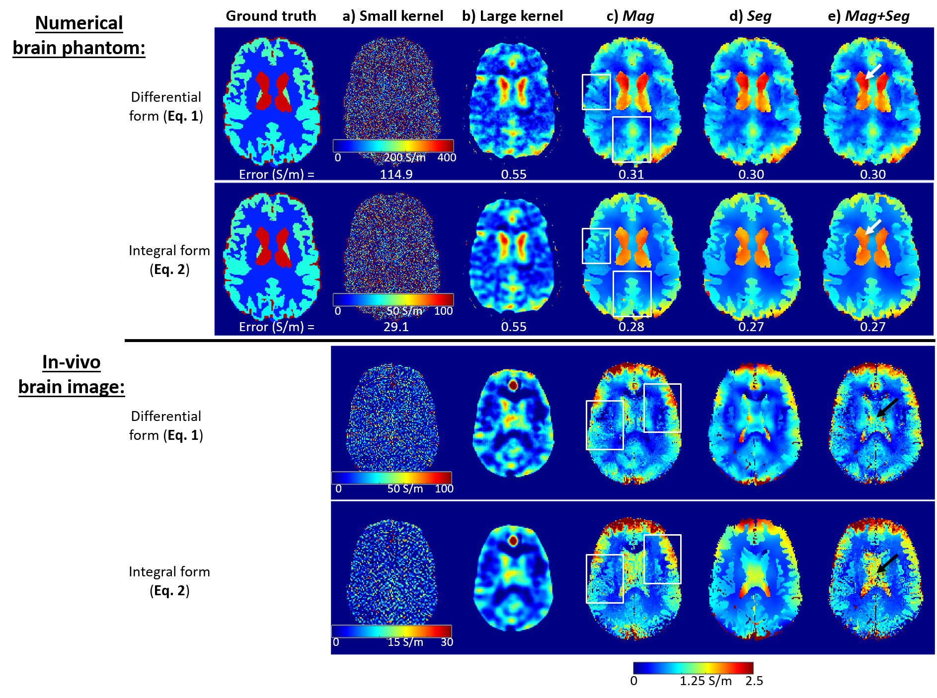
Figure 5 shows the optimised conductivity maps for the numerical phantom (top) and the in-vivo images (bottom). Compared to using a large kernel (5b), all conductivity maps had substantially improved edge preservation and errors using either Mag and/or Seg (5c-e). The integral-based approaches (5c-e) provided much sharper edges (white rectangles) and lower mean absolute errors than the differential-based methods, possibly because calculating the first derivatives amplifies the noise less (hence the smaller optimal kernel) than calculating the Laplacian. Increasing the kernel radius (for either the 3D quadratic fit or the surface integral) leads to inaccuracies even in the noise-free cases (Figures 3c and 4d). Therefore, the optimal kernel radii represent a trade-off between noise suppression and conductivity accuracy. Note that we optimised the kernel sizes throughout the brain which led to some additional conductivity underestimation in the ventricles (Figure 4c, white arrows) in exchange for more accurate GM conductivity (Figure 4c, black arrows). In the phantom, the ventricles were more attenuated when solving Equation 2 (Figure 5e, white arrows). This could be because the surface integral uses $$$\nabla\varphi_0$$$ values from the conductivity boundary (that the kernel follows for Mag+Seg) where the electromagnetic simulations were inaccurate (see boundary artifacts in $$$\nabla^2\phi_0$$$, Figure 3c arrows). On the contrary, the integral-based Mag+Seg approach provided the most realistic (i.e. highest) ventricle conductivity in vivo (Figure 5e, black arrows). Future work will repeat the experiment with $$$\phi_0=(\mu_0\omega)\cdot\nabla^{-2}\sigma$$$ providing a less realistic but boundary-artifact-free phantom.

Conclusions

Here, we developed, optimised, and compared different approaches for phase-based conductivity mapping in noisy images. We found that solving the integral-form (Equation 2) provided lower errors and better edge preservation in both simulated and in-vivo images. The integral-based approach with both magnitude- and segmentation-restricted kernels provided the best in-vivo conductivity map. All methods we developed are downloadable from https://xip.uclb.com/i/software/MRI_conductivity.html.

Acknowledgements

We would like to thank Dr Barbara Dymerska, Beata Bachrata, and Dr Simon Robinson for providing the in-vivo images. We are grateful to Dr Patrick Fuchs for his help with the electromagnetic simulations and Dr Ulrich Katscher for his insightful feedback.

Dr Anita Karsa and Dr Karin Shmueli were supported by European Research Council Consolidator Grant DiSCo MRI SFN 770939.

References

1. Katscher, Ulrich, and Cornelius AT van den Berg. "Electric properties tomography: biochemical, physical and technical background, evaluation and clinical applications." NMR in Biomedicine 30.8 (2017): e3729.

2. Liao, Yupeng, et al. "Correlation of quantitative conductivity mapping and total tissue sodium concentration at 3T/4T." Magnetic resonance in medicine 82.4 (2019): 1518-1526.

3. Tha, Khin Khin, et al. "Noninvasive electrical conductivity measurement by MRI: a test of its validity and the electrical conductivity characteristics of glioma." European radiology 28.1 (2018): 348-355.

4. van Lier, Astrid LHMW, et al. "Electrical properties tomography in the human brain at 1.5, 3, and 7T: a comparison study." Magnetic resonance in medicine 71.1 (2014): 354-363.

5. Lee, Joonsung, Jaewook Shin, and Dong‐Hyun Kim. "MR‐based conductivity imaging using multiple receiver coils." Magnetic resonance in medicine 76.2 (2016): 530-539.

6. Kim, Dong‐Hyun, et al. "Simultaneous imaging of in vivo conductivity and susceptibility." Magnetic resonance in medicine 71.3 (2014): 1144-1150.

7. Gho, Sung‐Min, et al. "Simultaneous quantitative mapping of conductivity and susceptibility using a double‐echo ultrashort echo time sequence: Example using a hematoma evolution study." Magnetic resonance in medicine 76.1 (2016): 214-221.

8. Fushimi, Motofumi, et al. " Morphology Enabled Quantitative Conductivity–Susceptibility Mapping with B1 and B0 Estimation from Complex Multi-echo Gradient Echo Signal." ISMRM 28th Annual Meeting, 8-14 August 2020.

9. Karsa, Anita, and Shmueli, Karin. “Simultaneous Noise Suppression and Edge Preservation in Phase-based MRI Conductivity Mapping.” Proceedings of the Annual Meeting of the ESMRMB. (2020).

10. Shin, Jaewook, et al. "Initial study on in vivo conductivity mapping of breast cancer using MRI." Journal of Magnetic Resonance Imaging 42.2 (2015): 371-378.

11. Voigt, Tobias, Ulrich Katscher, and Olaf Doessel. "Quantitative conductivity and permittivity imaging of the human brain using electric properties tomography." Magnetic Resonance in Medicine 66.2 (2011): 456-466.

12. Bulumulla, Selaka Bandara, Seung-Kyun Lee, and Teck Beng Desmond Yeo. "Calculation of electrical properties from B1+ maps-a comparison of methods." Brain 68.65.7 (2012): 66-2.

13. Katscher, Ulrich, et al. "Estimation of breast tumor conductivity using parabolic phase fitting." Adapting MR in a Changing World: ISMRM 20th Annual Meeting, Melbourne, Australia, 5-11 May 2012.

14. Dymerska, Barbara, et al. "Phase unwrapping with a rapid opensource minimum spanning tree algorithm (ROMEO)." Magnetic Resonance in Medicine (2020).

15. Eckstein, Korbinian, et al. "Computationally efficient combination of multi‐channel phase data from multi‐echo acquisitions (ASPIRE)." Magnetic resonance in medicine 79.6 (2018): 2996-3006.

16. Hammond, Kathryn E., et al. "Development of a robust method for generating 7.0 T multichannel phase images of the brain with application to normal volunteers and patients with neurological diseases." Neuroimage 39.4 (2008): 1682-1692.

17. https://www.fil.ion.ucl.ac.uk/spm/software/spm12/

18. Tustison, Nicholas J., et al. "N4ITK: improved N3 bias correction." IEEE transactions on medical imaging 29.6 (2010): 1310-1320.

19. Zubal, I. George, et al. "Two dedicated software, voxel-based, anthropomorphic (torso and head) phantoms." Proceeding of the International Conference at the National Radiological Protection Board. 1995.

20. Karsa, Anita, Shonit Punwani, and Karin Shmueli. "The effect of low resolution and coverage on the accuracy of susceptibility mapping." Magnetic resonance in medicine 81.3 (2019): 1833-1848.

21. Remis, Rob, and Edoardo Charbon. "An electric field volume integral equation approach to simulate surface plasmon polaritons." Advanced Electromagnetics 2.1 (2013): 15-24.

22. Chew, Weng Cho, Mei Song Tong, and Bin Hu. "Integral equation methods for electromagnetic and elastic waves." Synthesis Lectures on Computational Electromagnetics 3.1 (2008): 1-241.

23. Leijsen, Reijer, et al. "Developments in electrical-property tomography based on the contrast-source inversion method." Journal of Imaging 5.2 (2019): 25.

Figures

Figure 1: Descriptions of QCM methods based on the differential (top) and integral (bottom) equations used in this study and the optimised kernel radii. This is the first study that applies the methods labelled new.

Figure 2: The numerical phantom (top) and the in-vivo brain image (bottom). The noise-free B₁ phase (c) was calculated from realistic conductivity (a) and permittivity (b) distributions using electromagnetic simulations. Gaussian noise was added to the real and imaginary components of complex data created from (c) and the realistic phantom GRE magnitude (d) to match the SNR of the noisy phantom images (e-f) to that of the in-vivo data (h-i). GM/WM/CSF segmentations are displayed in (g) and (j).

Figure 3: Example kernel radius optimisation for solving Eq. 1 with the magnitude-based weighting approach. The mean absolute errors were calculated for kernel radii from 1 to 20 mm (a) and the minimum-error radius was selected as the optimum (a, cross). (b) shows example slices for some kernel sizes. The optimal kernel size provided the map most visually similar to the ground truth (b, yellow rectangle). An increasing kernel radius induces inaccuracies even in the noise-free phase map (c).

Figure 4: Example kernel radius optimisation for solving Eq. 2 with the magnitude-based weighting/restriction approach. The mean absolute errors were calculated for kernel radii from 1 to 20 mm (a) to find the minimum-error radius to estimate the first derivatives of the phase (b, yellow rectangle) and then the surface integral of the optimal first derivatives (c). An increasing kernel radius for step 2 induces inaccuracies even using the ground truth derivatives (d).

Figure 5: Optimised conductivity maps calculated using 10 different methods (from Figure 1) in the phantom (top) and in-vivo brain image (bottom). Mean absolute errors in the brain are also shown for the phantom. White rectangles highlight the superior performance of the integral-based methods. In the phantom, the integral-based methods seem to underestimate the ventricle conductivity more than the differential-based methods (white arrows), but the opposite is true in vivo (black arrows).

Proc. Intl. Soc. Mag. Reson. Med. 29 (2021)

3774