3773
Global and Direct Electrical Properties Tomography Method Based on the Linear Integral Equations for Impedivity
Motofumi Fushimi1, Naohiro Eda1, and Takaaki Nara1
1The University of Tokyo, Tokyo, Japan
1The University of Tokyo, Tokyo, Japan
Synopsis
The present paper introduces novel reconstruction methods for electrical properties tomography (EPT), in which conductivity and permittivity are reconstructed from the complex B1 field, and phase-based EPT, in which only conductivity is reconstructed from the B1 phase. The proposed methods reconstruct electrical properties (EPs) by solving a linear integral equation derived from Helmholtz's identity, and does not require calculation of the second-order derivatives of the measured data nor iterative updating of the estimates. Numerical simulations and phantom experiments showed that the proposed method could retrieve EPs more stably than the conventional method that solves a linear partial differential equation.
Introduction
Electrical properties tomography (EPT) reconstructs admittivity, namely conductivity and permittivity, which are useful in oncology and dosimetry, from B1 field data1. Conventional EPT methods can be divided into two types: partial-differential-equation-based (PDE-based) methods2,3,4 and integral-equation-based (IE-based) methods5,6. In this paper, we refer to these methods as local and global methods, respectively. Local methods are sensitive to noise due to numerical calculation of the Laplacian of the measured data, while global methods solve a nonlinear equation, possibly resulting in local minima. We previously proposed a direct and global method solving a linear IE of the electric field7. However, this method requires all the three components of the magnetic field $$$(H_{x},H_{y},H_{z})$$$, which are inaccessible in practical situations. In this paper, we propose a novel EPT method solving a linear IE for admittivity using only $$$H^{+}=(H_{x}+\mathrm{i}H_{y})/2$$$. We also propose a phase-based EPT method, in which conductivity is reconstructed from the measured B1 phase8, based on the same formulation. The proposed methods retrieve admittivity without calculating the Laplacian of the measured data, nor iteratively updating the estimate.Method
According to Hafalir et al.2, the following convection-reaction (cr) equation for impedivity $$$λ$$$ holds: $$λ{\Delta}H^{+}+{\nabla}λ\cdot\begin{pmatrix}2{\partial}H^{+}\\2\mathrm{i}{\partial}H^{+}\\\partial_{z}H^{+}\end{pmatrix}-\mathrm{i}ω_{0}μ_{0}H^{+}=0,\tag{1}$$ where $$$ω_{0}$$$ is Larmor's frequency, $$$μ_{0}$$$ is permeability of free space, and $$$\partial\equiv(\partial_{x}-\mathrm{i}\partial_{y})/2$$$. By introducing a new vector field $$$λ\nabla^{\mathrm{c}}H^{+}$$$, where $$$\nabla^{\mathrm{c}}\equiv\nabla-\mathrm{i}\nabla\times\hat{\boldsymbol{z}}$$$, Eq. (1) can be rewritten in a simple divergence-constraint form as follows: $$\nabla\cdot(λ\nabla^{\mathrm{c}}H^{+})=\mathrm{i}ω_{0}μ_{0}H^{+}.\tag{2}$$ Equation (2) is equivalent to the PDE derived in [4] to construct the modified finite difference (mFD) method.The cr/mFD method solves Eq. (1)/(2) using the finite element/difference method. In this paper, we derive a linear IE based on Helmholtz's identity by exploiting the fact that Eq. (2) is written in the divergence-constraint form.Helmholtz's identity9 states that a smooth vector field $$$\boldsymbol{f}$$$ defined in a bounded region of interest $$$Ω$$$ can be represented by its divergence and curl as follows: $$\boldsymbol{f}(\boldsymbol{r})=-\oint_{{\partial}Ω}{\nabla}G(\boldsymbol{r}^{\prime};\boldsymbol{r})(\boldsymbol{n}\cdot\boldsymbol{f})\mathrm{d}S^{\prime}+\int_{Ω}{\nabla}G(\boldsymbol{r}^{\prime};\boldsymbol{r})(\nabla\cdot\boldsymbol{f})\mathrm{d}V^{\prime}+\oint_{{\partial}Ω}{\nabla}G(\boldsymbol{r}^{\prime};\boldsymbol{r})(\boldsymbol{n}\times\boldsymbol{f})\mathrm{d}S^{\prime}-\int_{Ω}{\nabla}G(\boldsymbol{r}^{\prime};\boldsymbol{r})\times(\nabla\times\boldsymbol{f})\mathrm{d}V^{\prime},\tag{3}$$ where $$$G(\boldsymbol{r}^{\prime};\boldsymbol{r})=1/(4π\lvert\boldsymbol{r}^{\prime}-\boldsymbol{r}\rvert)$$$. By applying integration by parts to the last term of Eq. (3), we obtain $$\boldsymbol{f}(\boldsymbol{r})=-\oint_{{\partial}Ω}{\nabla}G(\boldsymbol{r}^{\prime};\boldsymbol{r})(\boldsymbol{n}\cdot\boldsymbol{f})\mathrm{d}S^{\prime}+\int_{Ω}{\nabla}G(\boldsymbol{r}^{\prime};\boldsymbol{r})(\nabla\cdot\boldsymbol{f})\mathrm{d}V^{\prime}+\int_{Ω}(\boldsymbol{f}\times\nabla)\times{\nabla}G(\boldsymbol{r}^{\prime};\boldsymbol{r})\mathrm{d}V^{\prime},\tag{4}$$ which represents a vector field using its divergence and itself instead of its curl. Here, substituting Eq. (2) into Eq. (4) yields $$λ\nabla^{\mathrm{c}}H^{+}=-\oint_{\partial Ω}{\nabla}G(\boldsymbol{r}^{\prime};\boldsymbol{r})(\boldsymbol{n}{\cdot}λ\nabla^{\mathrm{c}}H^{+})\mathrm{d}S^{\prime}+\int_{Ω}{\nabla}G(\boldsymbol{r}^{\prime};\boldsymbol{r})\mathrm{i}ω_{0} μ_{0}H^{+}\mathrm{d}V^{\prime}+\int_{Ω}(λ\nabla^{\mathrm{c}}H^{+}\times\nabla)\times{\nabla}G(\boldsymbol{r}^{\prime};\boldsymbol{r})\mathrm{d}V^{\prime}.\tag{5}$$ Given the EP values on $$${\partial}Ω$$$, the surface integrals can be calculated. Equation (5) is a linear IE for impedivity including only first-order derivatives of $$$H^{+}$$$, which can be calculated using the Savitzky-Golay filter10, and can be efficiently solved by the FFT-CG method11. In contrast to the previous method7,12 in which we derived an IE for $$$\boldsymbol{E}=λ\nabla\times\boldsymbol{H}$$$ which requires all components of $$$\boldsymbol{H}$$$, the proposed method considers $$$λ\nabla^{\mathrm{c}}H^{+}$$$ including only $$$H^{+}$$$ measured by the B1 mapping.
A similar formulation can be derived for phase-based EPT. According to Gurler et al.13, the following cr equation for resistivity, $$$ρ$$$, holds: $$ρ{\Delta}ϕ+{\nabla}ρ\cdot{\nabla}ϕ-2ω_{0}μ_{0}=0,\tag{6}$$ where $$$ϕ$$$ is the measured B1 phase. By introducing a vector field $$$ρ{\nabla}ϕ$$$, Eq. (6) can also be rewritten in divergence-constraint form as follows: $$\nabla\cdot(ρ{\nabla}ϕ)=2ω_{0}μ_{0}.\tag{7}$$ Substituting Eq. (7) into Eq. (2) yields $$ρ{\nabla}ϕ=-\oint_{{\partial}Ω}{\nabla}G(\boldsymbol{r}^{\prime};\boldsymbol{r})(\boldsymbol{n}{\cdot}ρ{\nabla}ϕ)\mathrm{d}S^{\prime}+\int_{Ω}{\nabla}G(\boldsymbol{r}^{\prime};\boldsymbol{r})2ω_{0}μ_{0}\mathrm{d}V^{\prime}+\int_{Ω}(ρ{\nabla}ϕ\times\nabla)\times{\nabla}G(\boldsymbol{r}^{\prime};\boldsymbol{r})\mathrm{d}V^{\prime}.\tag{8}$$ Equation (8) is a linear IE for resistivity including only first-order derivatives of $$$ϕ$$$, and can also be solved by the FFT-CG method.
We tested the proposed method by a numerical simulation and a phantom experiment and compared the obtained results with those of the cr methods. We constructed a sphere model for the simulation and a cylindrical phantom for the experiment as shown in Fig. 1. The simulation was performed by COMSOL Multiphysics 5.5 (COMSOL Inc.) and $$$H^{+}$$$ was obtained with a resolution of $$$1.4\times1.4\times5~\mathrm{mm^{3}}$$$. The experiment was conducted by the 3 T MR scanner Magnetom Prisma (Siemens) at the University of Tokyo and $$$H^{+}$$$ was obtained with a resolution of $$$1.4\times1.4\times10~\mathrm{mm^{3}}$$$. For the B1 mapping, we used the double angle method14.
Results and Discussion
Figure 2 shows the reconstructed conductivity and permittivity maps of the sphere model when no noise was added. The cr method gives the results with spurious oscillations arising from the unstable nature of the cr equation15. By introducing viscosity-type regularization15, the cr method yields stable but blurred results. In contrast, the proposed method yields accurate and stable results even without additional regularization. The proposed method has the least L2 error as shown in the table. Figure 3 shows the reconstruction results when 1% Gaussian noise was added. In the conventional method, strong regularization is required to stabilize the reconstruction, resulting in over-smoothed estimates. The proposed method yields stable results while preserving the edge. Figure 4 shows the conductivity maps reconstructed by phase-based EPT. Similar to EPT, the proposed method yields a more stable result than the conventional method while preserving the edge. Figure 5 shows the reconstructed conductivity maps of the cylindrical phantom. The reference map obtained by the conductivity meter (Hanna Instruments, HI8733) is shown in Fig 5(a). The proposed EPT method successfully reconstructed conductivity and a similar map is obtained by the proposed phase-based EPT method using only the B1 phase.Conclusion
We proposed novel EPT and phase-based EPT methods solving linear IEs for impedivity and resistivity derived from Helmholtz's identity. The proposed method could reconstruct EPs directly without second-order derivatives of the measured data. Numerical simulations and phantom experiments showed that the proposed method could retrieve EPs more robustly than the conventional method solving a linear PDE.Acknowledgements
This work was financially supported by Canon Medical Systems Corporation.References
- U.Katscher, T. Voigt, C. Findeklee, P. Vernickel, K. Nehrke, and O. Dössel, "Determination of Electric Conductivity and Local SAR Via B1 Mapping," IEEE Trans. Med. Imag., 28(9):1365-1374, 2009.
- F. S. Hafalir, O. F. Oran, N. Gurler, and Y. Z. Ider, "Convection-Reaction Equation Based Magnetic Resonance Electrical Properties Tomography (cr-MREPT)," IEEE Trans. Med. Imag., 33(3):777-793, 2014.
- H. Ammari, H. Kwon, Y. Lee, K. Kang, and J. K. Seo, "Magnetic-resonance-based reconstruction method of conductivity and permittivity distribution at Larmor frequency," Inv. Probl., 31(10):15001, 2015.
- C. Liu, J. Jin, L. Guo, M. Li, Y. Tesiram, H. Chen, F. Liu, X. Xin, and S. Crozier,"MR-based electrical property tomography using a modified finite difference scheme," Phys. Med. Biol., 63(14):145013, 2018.
- E. Balidemaj, C. A. T. van den Berg, J. Trinks, A. L. H. M. W. van Lier, A. J. Nederveen, L. J. A. Stalpers, H. Crezee, and R. F. Remis, "CSI-EPT: A Contrast Source Inversion Approach for Improved MRI-Based Electric Properties Tomography," IEEE Trans. Med. Imag., 34(9):1788-1796, 2015.
- R. L. Leijsen, W. M. Brink, C. A. T. van den Berg, A. G. Webb, and R. F. Remis, "3-D Contrast Source Inversion-Electrical Properties Tomography," IEEE Trans. Med. Imag., 37(9):2080-2089, 2018.
- N. Eda, M. Fushimi, K. Hasegawa, and T. Nara, "Noniterative Electrical Properties Tomography Reconstruction Method Based on Three-Dimensional Integral Equation for the Electric Field," Proc. ISMRM 28th Annual Meeting, 3191, Aug. 2020.
- T. Voigt, U. Katscher, and O. Dössel, "Quantitative Conductivity and Permittivity Imaging of the Human Brain Using Electric Properties Tomography," Magn. Reson. Med., 66(2):456-466, 2011.
- Y. F. Gui, and W.-B. Dou, "A Rigorous and Completed Statement on Helmholtz Theorem," PIER, 69:287-304, 2007.
- A. Savitzky, and M. J. E. Golay, "Smoothing and Differentiation of Data by Simplified Least Squares Procedures," Anal. Chem., 36(8):1627-1639, 1964.
- M. F. Cátedra, J. G. Cuevas, and L. Nuno, "A scheme to analyze conducting plates of resonant size using the conjugate-gradient method and the fast Fourier transform," IEEE Trans. Antennas Propag., 36(12):1744-1752, 1988.
- N. Eda, M. Fushimi, and T. Nara, Proc. ISMRM 29th Annual Meeting, 1438, May 2021.
- N. Gurler, and Y. Z. Ider, "Gradient-Based Electrical Conductivity Imaging Using MR Phase," Magn. Reson. Med., 77(1):137-150, 2017.
- E. K. Insko, and L. Bolinger, "Mapping of the Radiofrequency Field," J. Magn. Reson. A, 103(1):82-85, 1993.
- C. Li, W. Yu, and S. Y. Huang, "An MR-Based Viscosity-Type Regularization Method for Electrical Property Tomography", Tomography, 3(1):50-59, 2017.
Figures
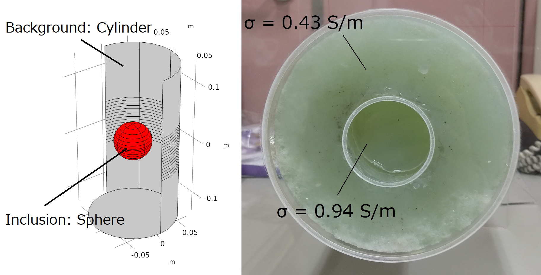
Figure1: (left) The sphere model used in the numerical simulation and (right) the cylindrical phantom used in the phantom experiment. Conductivity values of the phantom were obtained by a conductivity meter.
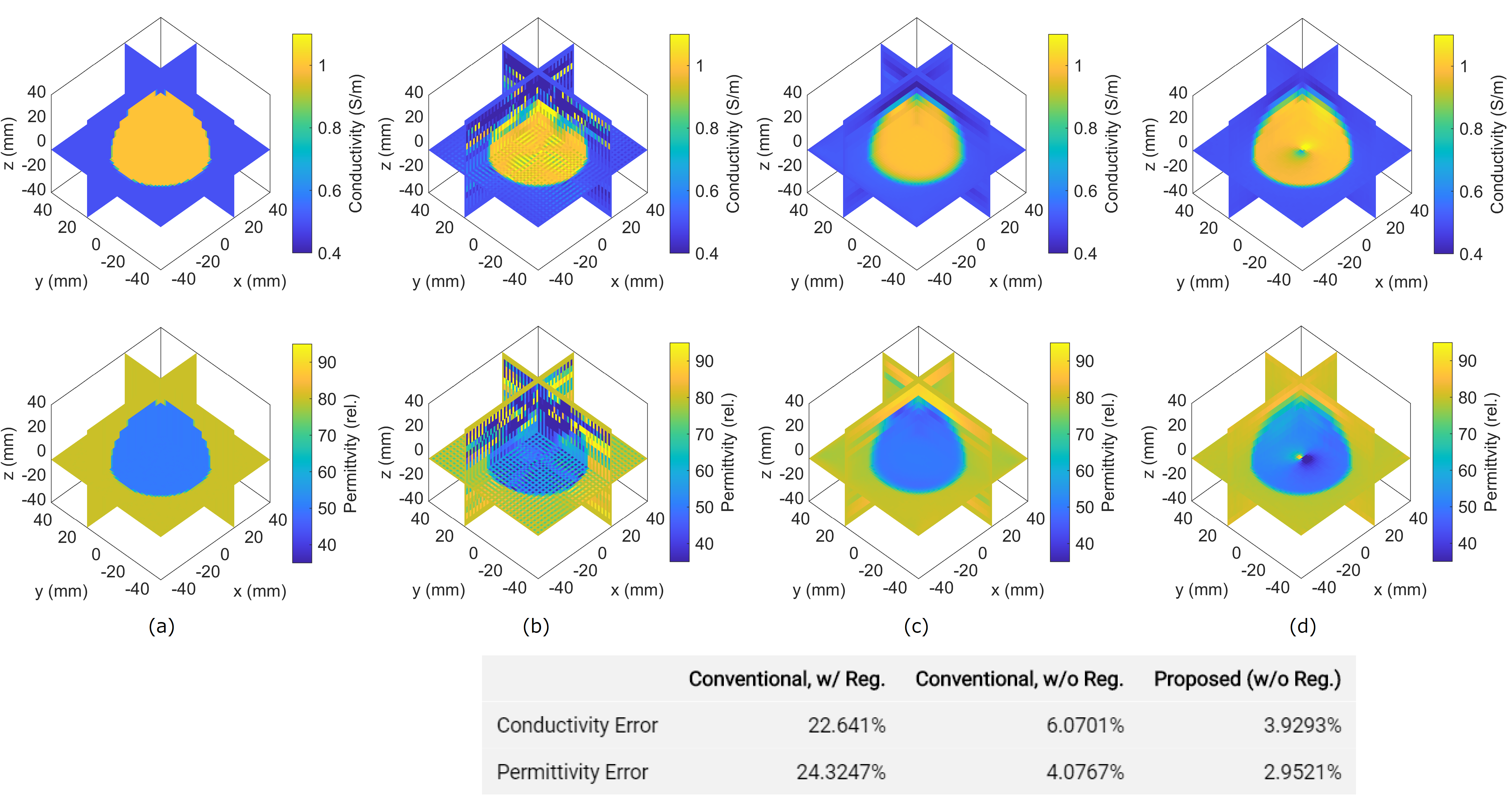
Figure 2: Conductivity and permittivity maps for the sphere model when no noise is added. (a) True maps and reconstruction results of (b) the conventional method with no regularization, (c) the conventional method with viscosity-type regularization, and (d) the proposed method with no regularization. The table at the bottom shows the normalized L2 errors of each method.
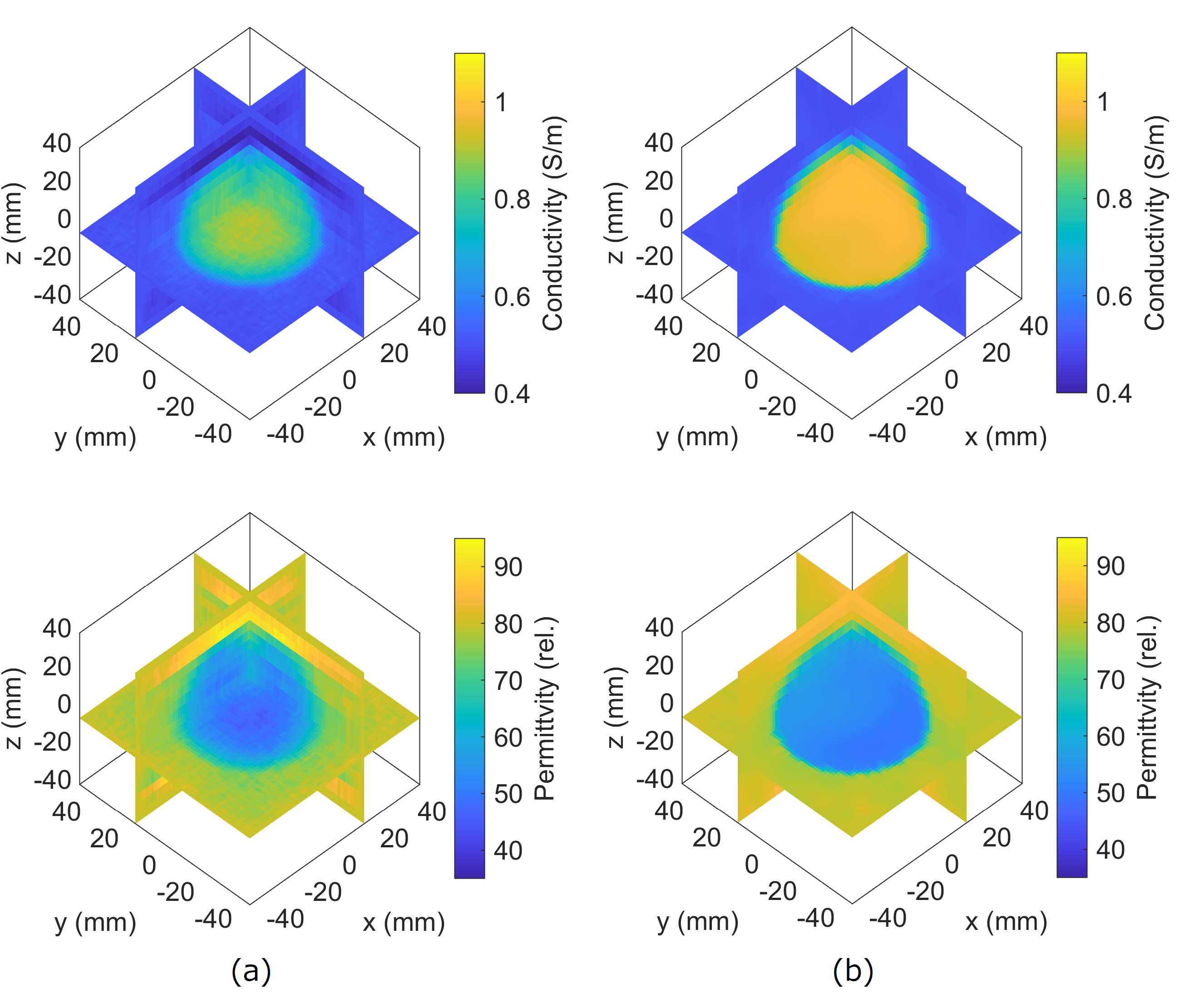
Figure 3: Conductivity and permittivity maps for the sphere model when 1% Gaussian noise is added. The reconstruction results of (a) the conventional method with viscosity-type regularization, and (b) the proposed method with TV regularization.
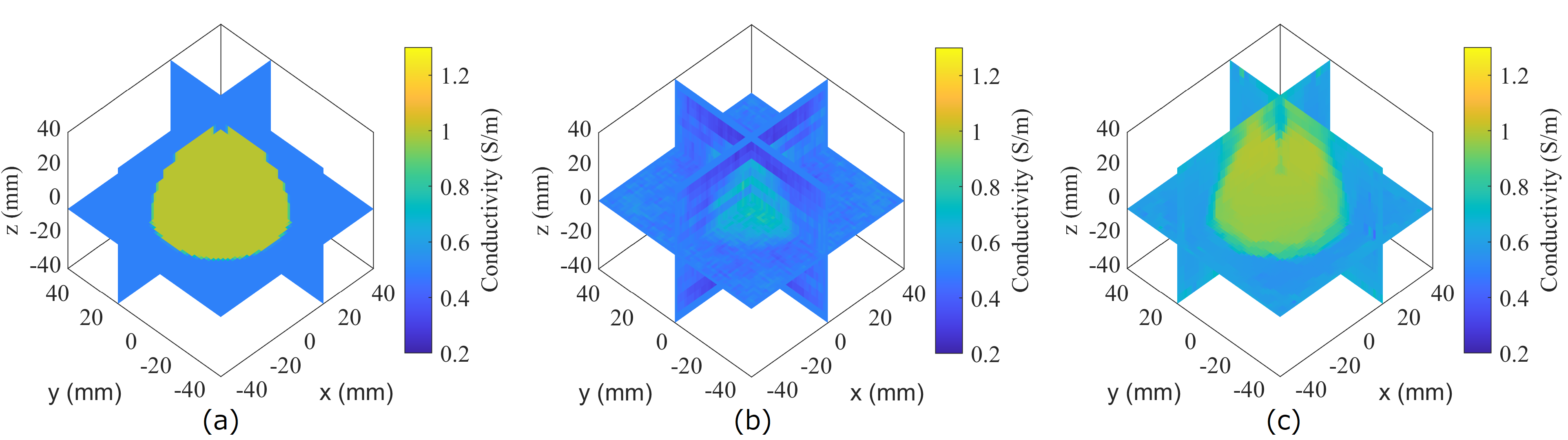
Figure 4: Conductivity maps obtained by phase-based EPT reconstruction for the sphere model when 1% Gaussian noise is added. (a) True map, (b) reconstruction results of the conventional method with viscosity-type regularization, and (c) reconstruction results of the proposed method with TV regularization.
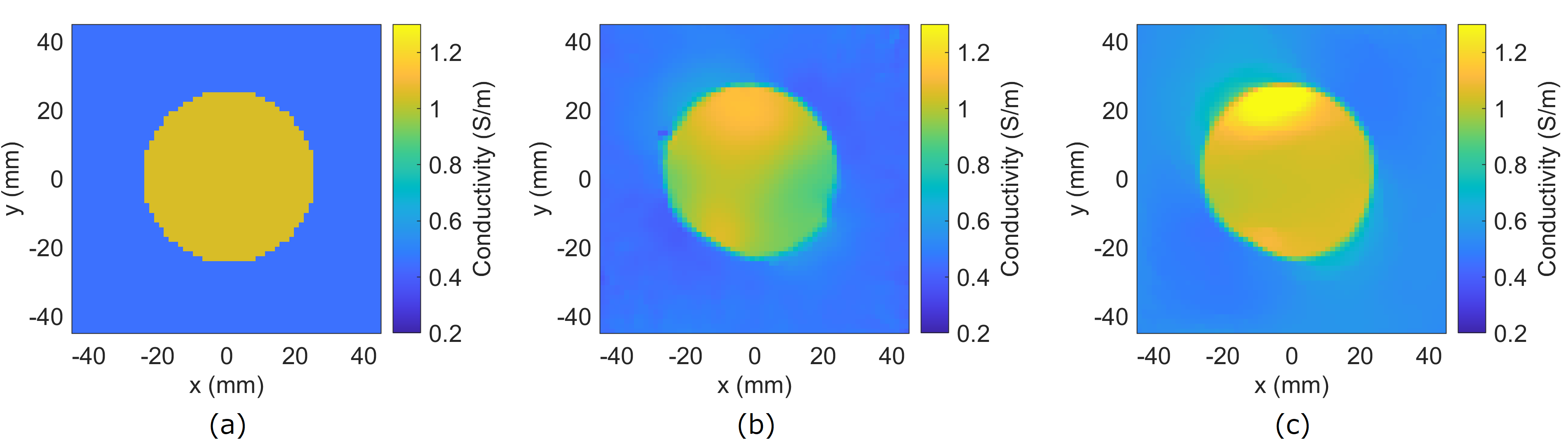
Figure 5: Conductivity maps obtained by EPT and phase-based EPT reconstruction for the cylindrical phantom. (a) Reference map obtained by a conductivity meter, and the reconstruction results of the proposed (b) EPT and (c) phase-based EPT methods with TV regularization.