Introduction

MR images can vary considerably across sites and along time, due to differences in experimental conditions, sequence implementation details, and image reconstruction and post-processing choices. To make MRI-derived measures — and research findings based on them — more reproducible, a significant amount of effort has gone into developing open software tools for image reconstruction and post-processing, for a wide range of applications including functional MRI and quantitative imaging. Recently, significant progress has also been made toward making the data acquisition itself more consistent across sites and vendor platforms, by introducing an abstraction layer that allows an MRI experiment to be fully encapsulated in a vendor-agnostic container and ported directly to the scanner for execution [1-3].
B0 shimming, being one of the first steps of the routine MRI workflow, has been so far overlooked in the abovementioned cross-platform harmonization efforts. B0 inhomogeneity is a major source of image artifacts and site-to-site variability in MRI, particularly for sequences that employ long data readout duration (e.g., EPI) and/or long echo times (TE). Commercial MRI scanners are typically equipped with linear and 2nd-order (spherical harmonic) shim channels that offer some control of the B0 field, but the shim settings are usually adjusted automatically and non-transparently during the scanner’s prescan routine with little or no user input. In fact, some built-in shim adjustment routines only adjust the linear shims and do not take full advantage of the hardware capabilities present. This practice makes it difficult to ensure consistent experimental conditions across sessions and sites, and may lead to suboptimal shim settings for a given application.
Fortunately, vendors typically expose a command-line interface for manually setting the shim currents. In this work we propose to exploit those interfaces by introducing an open toolbox for high-order shim optimization that can be employed across sites and vendor platforms.

Methods

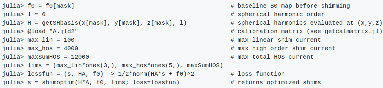
Software tool: The shim optimization tool is written in Julia, an open programming language that is available on all major computing platforms. We use the NLopt.jl package to construct a general nonlinear optimizer that takes as input the spatial shim patterns (‘H*A’ in Fig. 1) and the baseline B0 fieldmap we wish to shim, both evaluated at the spatial locations (mask) we wish to shim over. The function returns the optimized shims over the masked region, subject to shim current constraints. ‘H’ is a matrix containing spherical harmonic basis functions evaluated within the mask locations. ‘A’ is a small matrix containing spherical harmonic expansion coefficients for each shim channel, and is described further below.
Experimental validation: We evaluated the shim optimizer at two different sites, each housing a 3T MRI scanner equipped with 2nd-order shim coils (GE MR750 and Siemens Prisma). On each system, we first calibrated the B0 fields produced by each linear and 2nd-order shim channel (not shown), using either a built-in 3D GRE sequence or a similar sequence implemented in Pulseq [2]. These calibration data need to be obtained only once for each site. We then fit each map to a spherical harmonic basis of order l = 2 or higher and saved the expansion coefficients in a calibration matrix `A` that is unique to each scanner.
At Site 1, we performed two shim experiments: first we performed global 2nd-order shimming in a homogeneous cylindrical agar phantom placed upright inside an 8-channel head coil. We then performed localized 2nd-order shimming in an anthropomorphic head phantom placed in a birdcage Tx/Rx coil. At Site 2, we obtained B0 field maps in a spherical agar phantom before and after running the built-in 2nd-order shim routine, and compared that result with the predicted B0 map using optimized shims obtained with the proposed toolbox. All experiments used a least-squares loss function. At Site 1, the built-in routine optimized the linear shim coils globally, while at Site 2 both the 1st- and 2nd-order shims were optimized (also globally) by the built-in routine.

Results

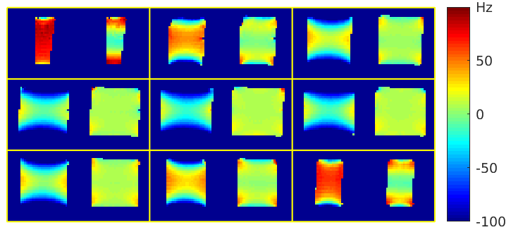
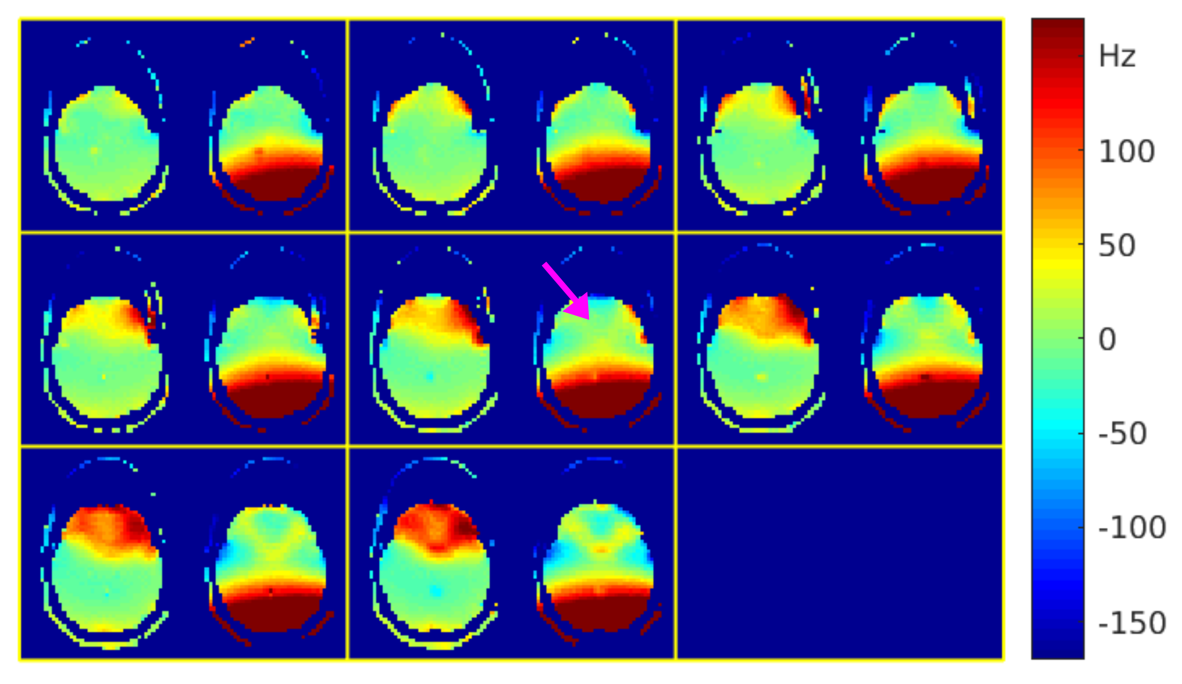
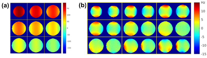
Figures 2 and 3 show the acquired B0 field maps before and after applying the proposed shim tool at Site 1. In Fig. 2, the mask contained the entire object, whereas in Fig. 3 the mask contained a local region in the frontal ‘cortex’ that exhibits significant B0 inhomogeneity prior to 2nd-order shimming. Figure 4 shows that the global built-in 2nd-order shim routine at Site 2 is in good agreement with the shims output by the proposed toolbox.

Conclusion

We have introduced a simple, general, and flexible software tool that allows B0 shims to be set in a consistent and controlled way across sites and vendor platforms. The framework allows for nonlinear loss functions, and may be useful for exploring alternative shimming criteria (beyond least-squares) in the future. We envision this tool as one component of a more harmonized MRI workflow in support of reproducible MRI research.

Acknowledgements

This work was supported by NIH Grants R21EB019653, R21AG061839, R01MH119222, R01 EB023618, R01 EB028797, U01 EB025162, P41 EB030006, U01 EB026996.