3760
PyPulseq in a web browser: a zero footprint tool for collaborative and vendor-neutral pulse sequence development
Keerthi Sravan Ravi1,2, John Thomas Vaughan Jr.2, and Sairam Geethanath2
1Biomedical Engineering, Columbia University, New York, NY, United States, 2Columbia Magnetic Resonance Research Center, New York, NY, United States
1Biomedical Engineering, Columbia University, New York, NY, United States, 2Columbia Magnetic Resonance Research Center, New York, NY, United States
Synopsis
PyPulseq is a free, open-source and vendor-neutral pulse sequence development (PSD) tool, allowing users to develop MR sequences using the Python programming language. This work demonstrates running PyPulseq in a web browser. This is accomplished by leveraging Google Colab which enables executing arbitrary code in a web browser. A single-slice 2D Gradient Recalled Echo pulse sequence is programmed and executed on a 3T scanner and the acquired data is visualized. PyPulseq on Colab enables portable PSD. It is beneficial for educational purposes, collaborative PSD and for fostering reproducible acquisition methods.
Introduction
Conventionally, designing MR pulse sequences has required knowledge of vendor-specific pulse sequence development (PSD) environments. Pulseq [1] has enabled open-source vendor-neutral PSD. Pulse sequences designed using Pulseq can be executed on Siemens, GE or Bruker hardware with the aid of vendor-specific interpreters. However, the MATLAB-associated licensing cost required to leverage Pulseq is prohibitive. PyPulseq [2, 3] enables free, open-source and vendor-neutral PSD on the Python programming language (Figure 1, shown in blue). Users can install PyPulseq via a single command and begin designing pulse sequences. Google (Alphabet Inc., Mountain View, CA, USA) recently launched Colab - an collaborative Python programming tool that runs in a supported web browser (http://colab.research.google.com). Users can program arbitrary code in code cells, and execute a collection of these cells as a Colab notebook. This work introduces PyPulseq on Colab, enabling collaborative and zero footprint development, rapid debugging and deployment of pulse sequences (Figure 1, shown in orange). It also fosters reproducible acquisition methods [4, 5]. A 2D Gradient Recalled Echo (GRE) pulse sequence is programmed, exported and executed on a Siemens Prisma Fit 3T scanner. The acquired data is reconstructed offline and presented for visualization purposes.Methods
A 2D GRE pulse sequence was programmed across nine code cells. Text cells were inserted to present relevant information and to demarcate sections such as defining constants, defining events, constructing the pulse sequence, plotting and lastly exporting. First, a new Colab notebook was created. The prerequisite PyPulseq library was installed and imported in cells 1 and 2 (Figure 3). In cell 3, user-defined constants such as the number of frequency and phase encodes, slice thickness, field of view, etc. were defined. A variable defining the hardware limits and a corresponding sequence object was created in cell 4. These include maximum gradient strength, maximum slew rate and radiofrequency ringdown time among others (Figure 3a). Time constants such as echo time and repetition time were declared in cell 5. PyPulseq supports arbitrary-, Gauss-, sinc- and rectangular-shaped radiofrequency (RF) pulses. For spatially varying magnetic field gradients, it supports arbitrary- and trapezoid-shaped envelopes. These built-in functions were leveraged to program the individual components of the pulse sequence such as the RF pulse, the slice-select gradient, phase-encoding gradient, delays etc. across cells 6-10 (Figure 3b). Finally, all these components were assembled to construct a sequence object in cell 11 (Figure 3c). The sequence object represented a single-slice 2D GRE sequence. The pulse timing diagram was plotted for visual inspection in cell 12 (Figure 3c). For clarity, only the first 20 milliseconds of the pulse timing diagram, as indicated by the ‘time_range’ parameter in the ‘PLOTTING TIMING DIAGRAM’ block were visualized, as shown in Figure 3. Finally, the sequence object was exported as a .seq file using PyPulseq’s built-in method in cell 14. The pulse sequence was executed on a Siemens Prisma Fit 3T to image the ISMRM phantom. The acquired data was reconstructed offline for visualization purposes.Results
Google Colab enables combining plain-text and arbitrary code via the use of text cells and code cells respectively. Additionally, a text cell supports embedded images and GIF animations. This allows users to present relevant information useful for tutorials, for example. Examples of this can be observed across all parts of Figure 3: each component of the pulse sequence is delimited by a text block that presents a one-line description of the purpose of the associated code block(s). Figure 5 presents the reconstruction of the acquired data. Google Colab notebooks can be shared publicly on the internet. Recipients can edit or make copies of the notebooks. All of these features combined facilitate the creation of rich-tutorials that are suitable for educational purposes, and foster collaborative development, debugging and deployment of pulse sequences.Discussion and conclusion
As illustrated in Figure 1, PyPulseq already enabled vendor-neutral PSD with zero associated licensing costs. The flexibility to install and run PyPulseq on Google Colab is an additional benefit. For the first time to the best of our knowledge, users can leverage a collaborative PSD solution. This enables multi-site PSD, multi-site trials of identical implementations, rapid prototyping and collaborative debugging of pulse sequences, and allows reproducibility of acquisition methods. Future work involves incorporating image reconstruction tools inline, which will be bolstered by Colab’s GPU/TPU hardware accelerators. Google Colab’s ability to allow users to upload files or access files stored on Google Drive cloud storage, built-in support for GPU acceleration will simplify the image reconstruction workflow. In conclusion, this work demonstrates leveraging PyPulseq and Google Colab to deliver an open-source, free to use, web based, portable pulse sequence development tool.Acknowledgements
This study was funded [in part] by the Seed Grant Program for MR Studies and the Technical Development Grant Program for MR Studies of the Zuckerman Mind Brain Behavior Institute at Columbia University and Columbia MR Research Center site.References
- Layton, Kelvin J., et al. "Pulseq: a rapid and hardware‐independent pulse sequence prototyping framework." Magnetic resonance in medicine 77.4 (2017): 1544-1552.
- Ravi, Keerthi Sravan, et al. "Pulseq-Graphical Programming Interface: Open source visual environment for prototyping pulse sequences and integrated magnetic resonance imaging algorithm development." Magnetic resonance imaging 52 (2018): 9-15.
- Ravi, Keerthi Sravan, Sairam Geethanath, and John Thomas Vaughan. "PyPulseq: A Python Package for MRI Pulse Sequence Design." Journal of Open Source Software 4.42 (2019): 1725.
- Stodden, Victoria. "Reproducible research for scientific computing: Tools and strategies for changing the culture." Computing in Science & Engineering 14.4 (2012): 13-17.
- Goodman, Steven N., Daniele Fanelli, and John PA Ioannidis. "What does research reproducibility mean?." Science translational medicine 8.341 (2016): 341ps12-341ps12.
Figures
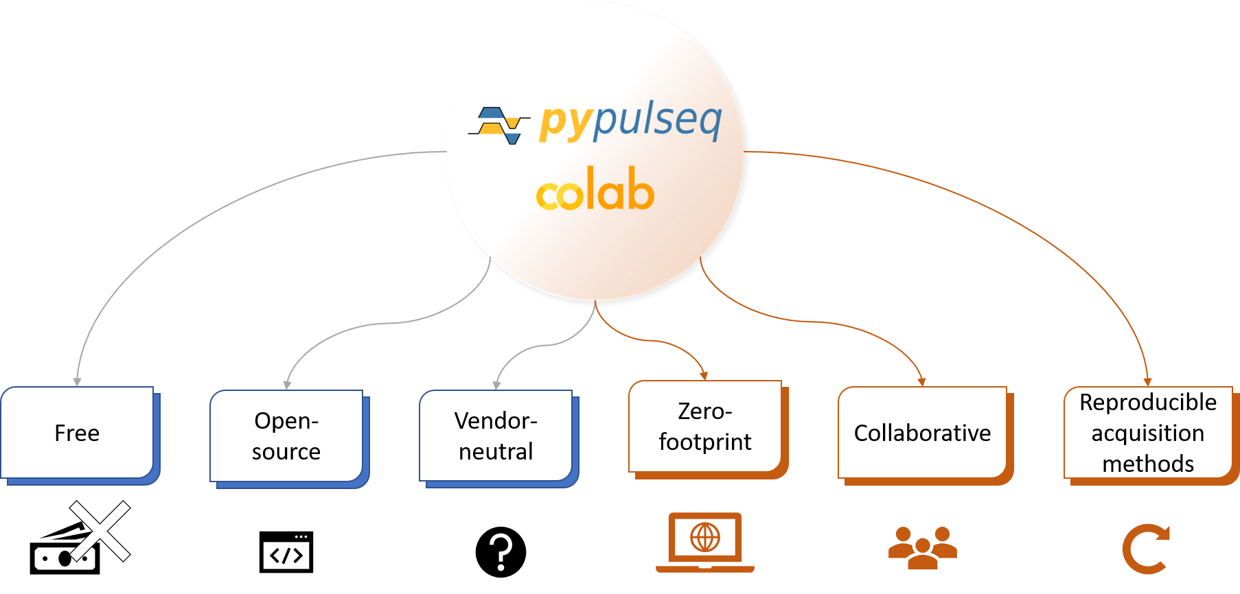
Figure 1. PyPulseq on Google Colab enables zero footprint and collaborative Pulse Sequence Development (PSD). PyPulseq enables free, open-source and vendor-neutral PSD (shown in blue). The ability to run PyPulseq on a browser via Google Colab enables multi-site PSD, multi-site trial of identical implementations, rapid prototyping and debugging of pulse sequences, and fosters reproducible acquisition methods (shown in orange).
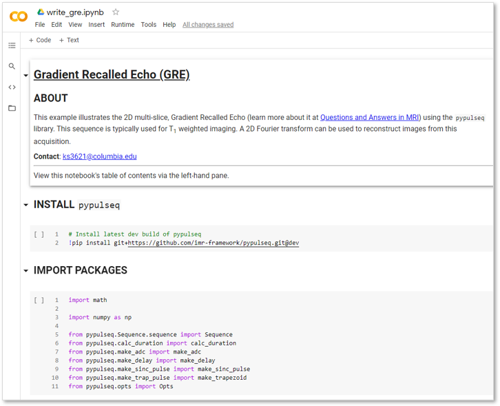
Figure 2. Screenshot of installing the prerequisite PyPulseq library and importing the required packages. The ‘about’ section of the Colab notebook links to a reputable resource where users can learn more about the sequence. In the ‘install’ section, PyPulseq is installed from Github via a single command. The ‘import’ section details the specific components that are leveraged in constructing the 2D Gradient Recalled Echo sequence.
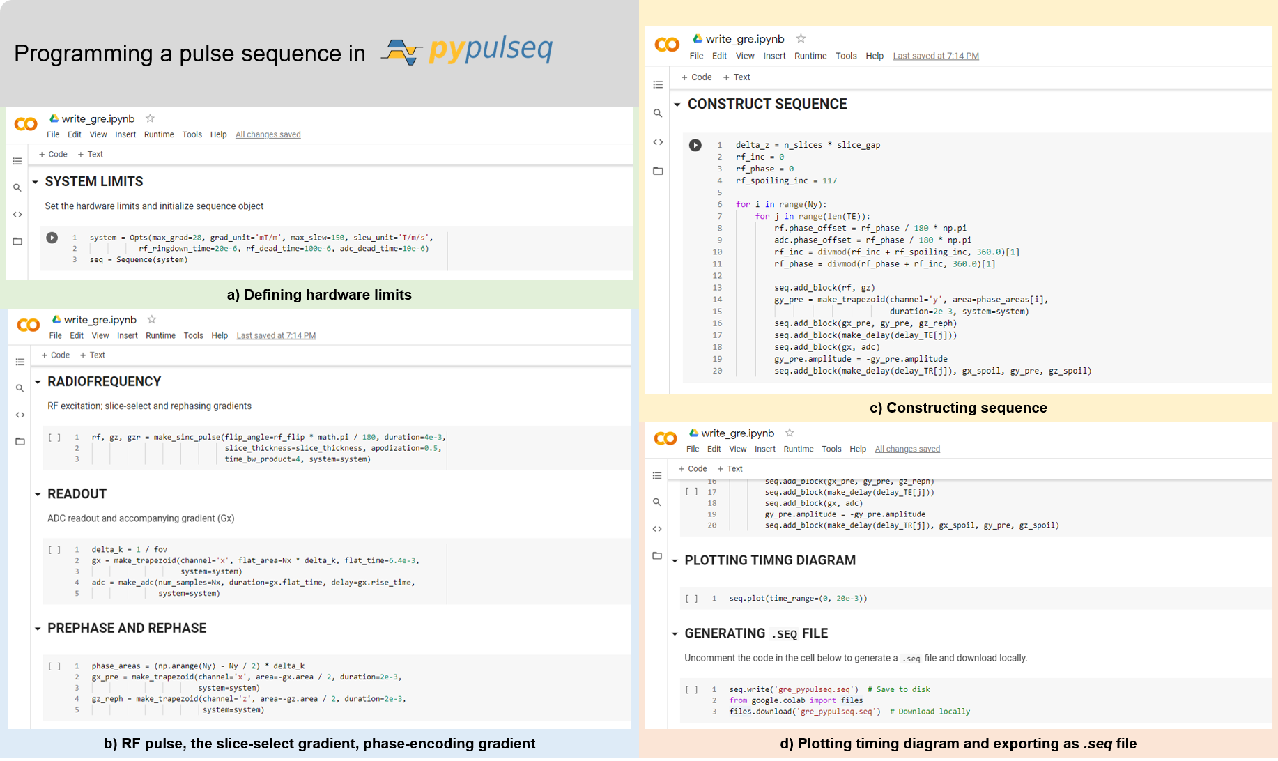
Figure 3. Programming a sequence in PyPulseq. (a) The hardware limits of the system intended to be executed on are set (for example maximum gradient strength, maximum slew rate, etc.). (b) The individual pulse sequence components such the radiofrequency pulse, analog-to-digital readout, etc. are defined. (c) These components are subsequently assembled to form a ‘sequence’ object representing the pulse sequence. (d) The pulse timing diagram is visualized and the sequence is exported as a .seq file.
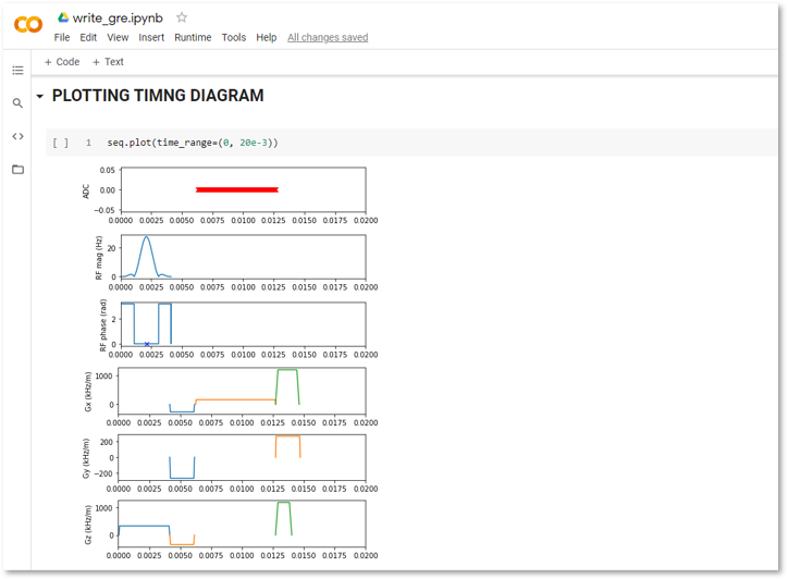
Figure 4. Pulse timing diagram of the 2D Gradient Recalled Echo sequence. For clarity, only the first 20 milliseconds of the pulse timing diagram was visualized.
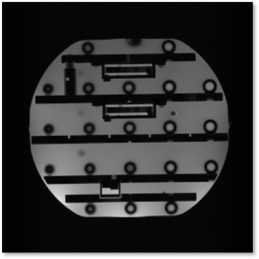
Figure 5. Reconstruction of data acquired imaging an ISMRM phantom. A single-slice 2D Gradient Recalled Echo sequence was designed using PyPulseq on Colab. The sequence was then exported as a .seq file and executed on a Siemens Prisma Fit 3T scanner. The acquired data was reconstructed using a 2D Fourier transform.