3733
Robust and Generalizable Quality Control of Structural MRI images1Subtle Medical Inc., Menlo Park, CA, United States
Synopsis
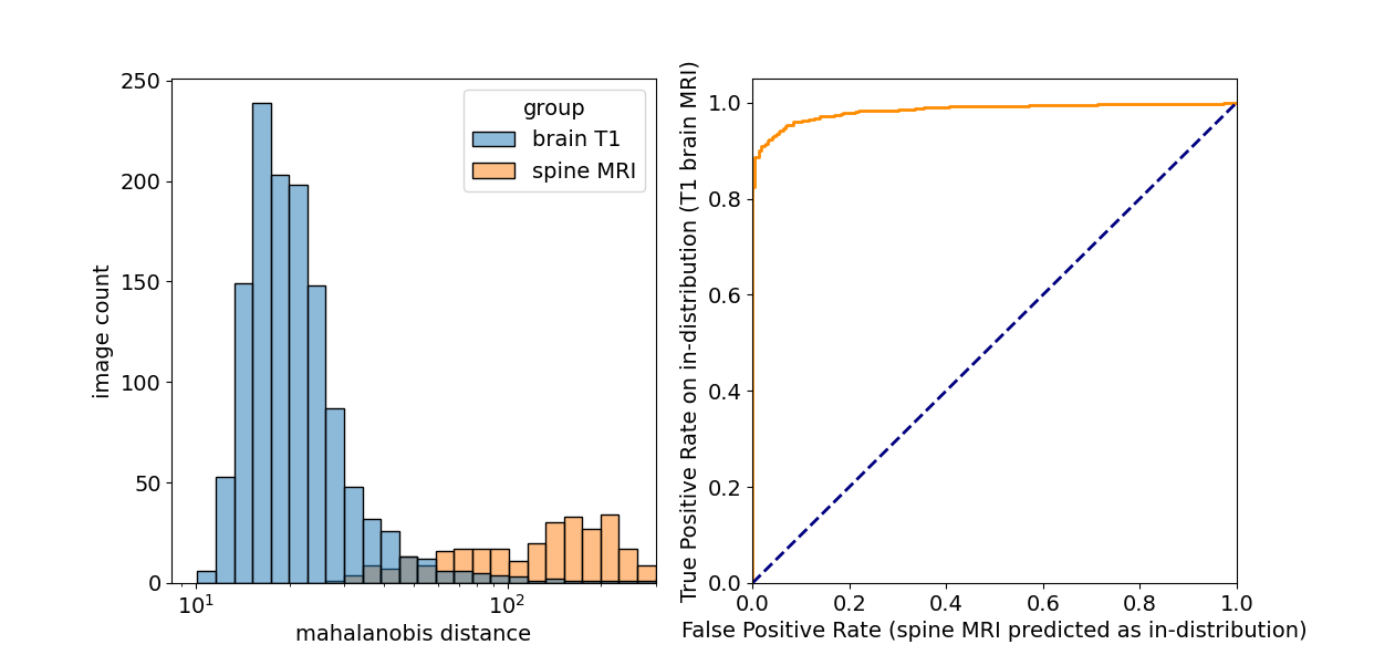
We present an automated deep learning-based quality control system that generalizes to images of different orientations, images with and without contrast as well as those from different acquisition sites. Because the same model was able to classify images with different orientations, test-time augmentation substantially improved performance. Images that were moderately affected by artifacts were able to be identified with 95% accuracy. Furthermore, robustness to different data types (and potentially artifact types) was ensured by using an out-of-distribution detection procedure. This was able to discriminate spine MRI images from T1 brain images with an AUC of 0.98.
Introduction
Subject motion during MRI acquisition is the most common cause of MRI quality degradation. Recent studies have suggested that deep learning (DL) can be effective for automatic MRI quality control (QC). While promising, the generalizability of DL-based QC to scan orientation and parameters, scanner types, as well as the use of contrast agent has not yet been thoroughly studied. This study aims to develop and evaluate a DL-based automated motion artifact detection system in the aforementioned generalized clinical settings. In addition, robustness is ensured through out-of-distribution detection as a safeguard against new data types that are not part of the training set.Methods
Datasets: Three separate 3D T1-weighted brain databases were used (two publicly available: IXI1 and OpenNeuro2, and 1 in-house). These contained images of diverse clinical indications from multiple scanner manufacturers and sites, all 3 orientations (axial, coronal, sagittal), images with and without gadolinium contrast agent. All three datasets were used across training, validation and testing. The test set also contained n=15 images from a new site not included in the training or validation sets.Labelling: Based on an in-house quality control protocol, MRI volumes were manually assessed on a 5-point Likert scale for severity of subject motion, with 5 being artifact free and 1 being severely corrupted. A quality score below 4 was considered to have failed QC.
Training: n=1829 (166 failures) volumes. Validation: n=1265 were used for hyperparameter optimization. Testing: n=37 images independently scored by two board certified radiologists. Out-of-distribution: An in-house dataset of (n=296) spine MRIs was used to assess performance of the out-of-distribution (OOD) detection classifier.
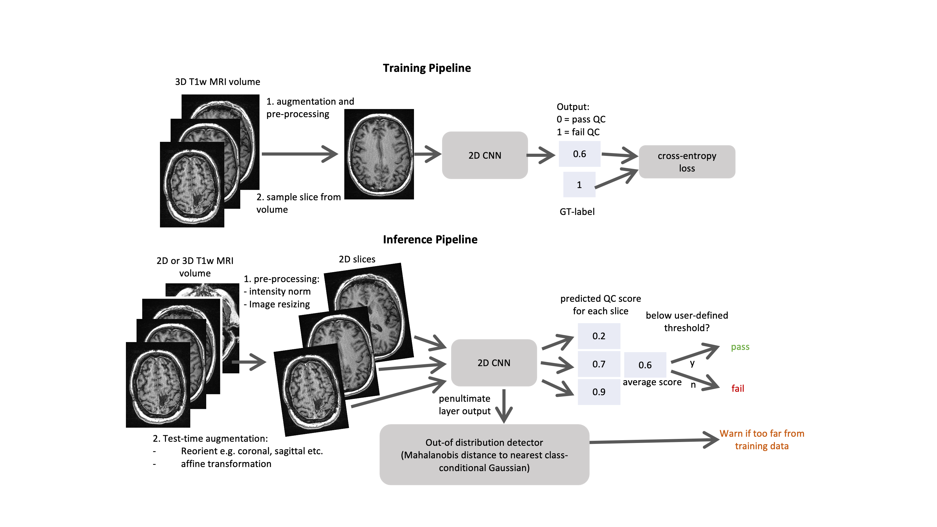
Model Design and training: The training and inference workflows are outlined in Fig. 1. A 2D EfficientNetB03 was trained using cross-entropy loss to predict a QC score for each slice (with 0=pass and 1=fail). For the inference workflow, test-time augmentation was carried out using reorientations and affine transformations. Volume-wise predictions were generated using the mean quality score across all slices. OOD detection was carried out by outputting the penultimate layer from the 2D CNN and using the Mehalanobis distance to the nearest class conditional distribution4.
Performance Evaluation: Due to class imbalance, average precision was used as the primary evaluation metric. Area-under-the receiver operator curve (AUC) was used for OOD detection evaluation. Performance was compared against a baseline classifier which scored all images as ‘pass’ QC. Images were considered QC success/failure based on radiologists’ scores (score < 3 or 4).
Results
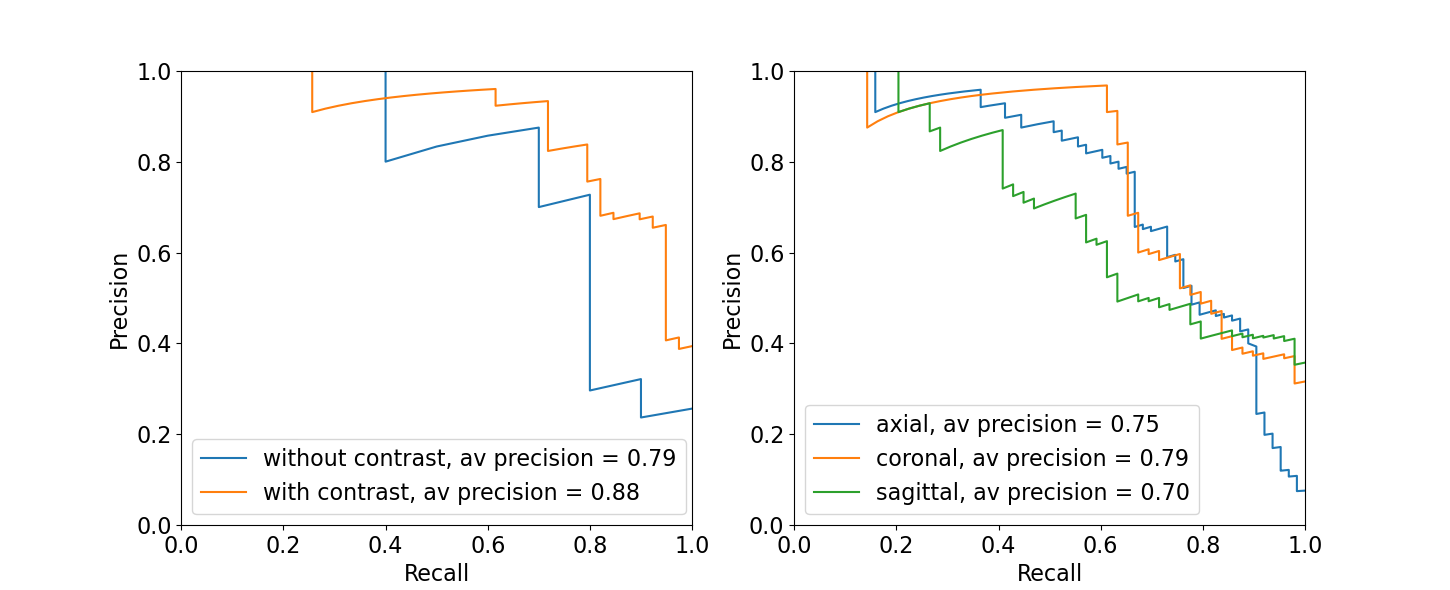
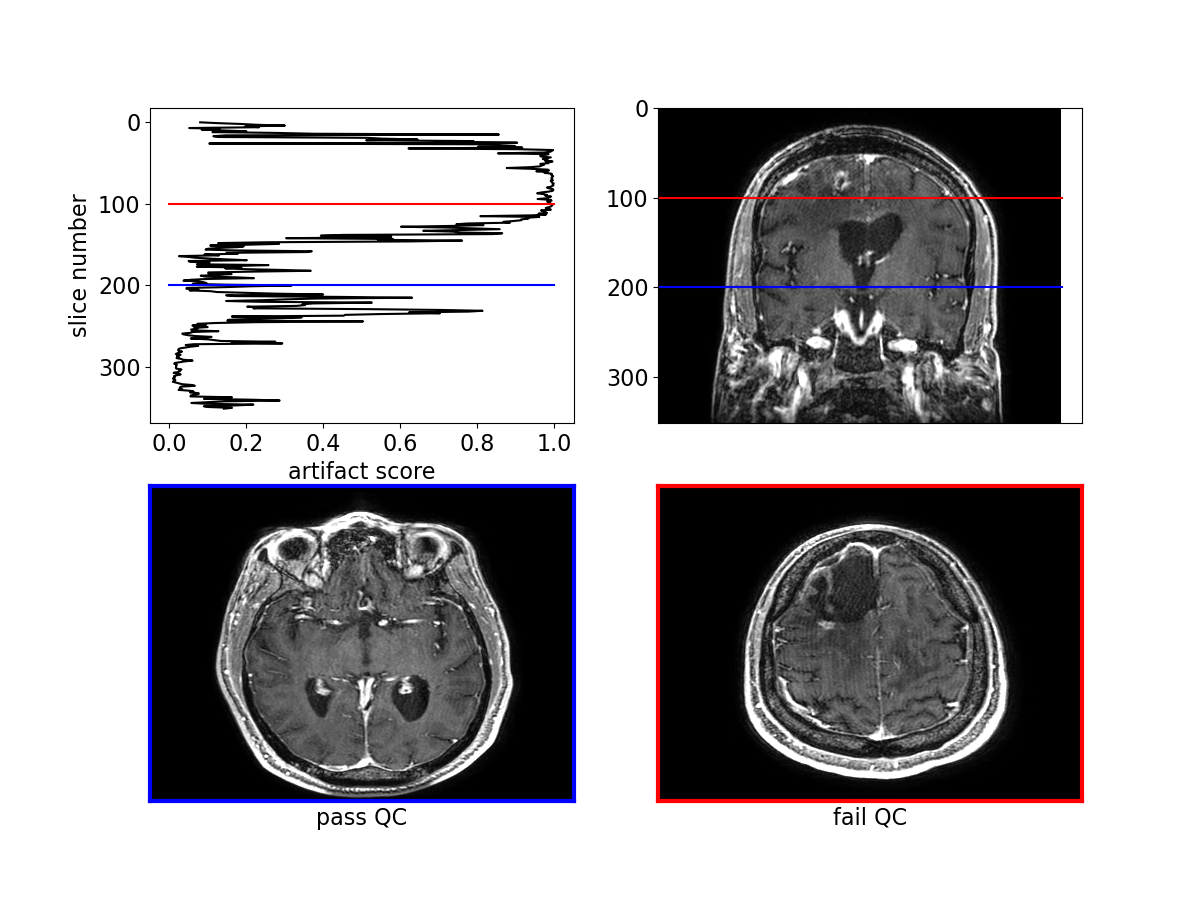
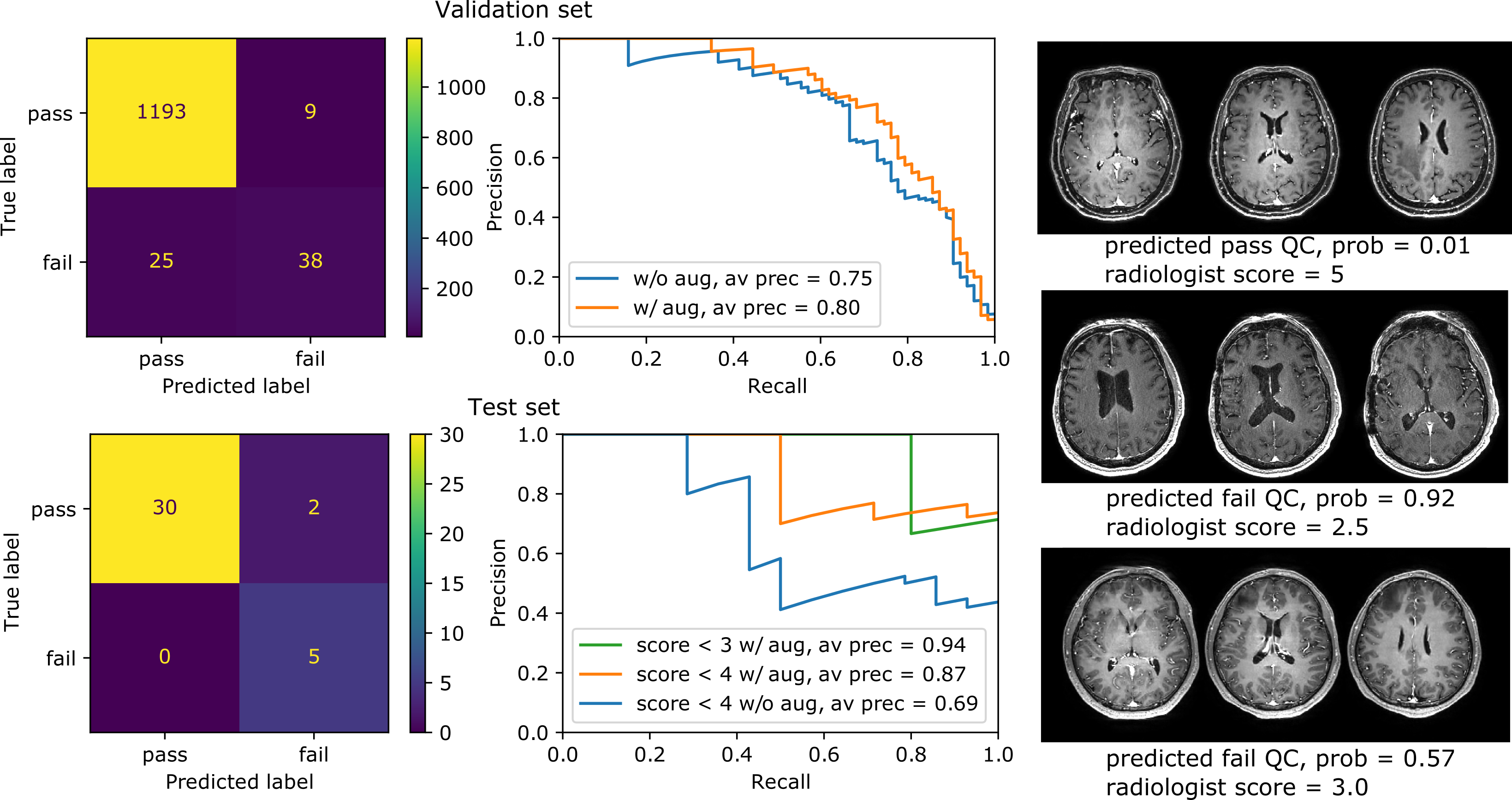
The algorithm performed well on images with and without gadolinium contrast agent (average precision = 0.79 vs. 0.88 respectively). In addition, training on the axial, coronal and sagittal views, meant the same model was also robust to resampling the same images in different orientations. For example, the average precision on axially acquired images was 0.75 and applying the model on the coronal and sagittal views resulted in comparable average precisions of 0.79 and 0.7 respectively (Fig. 2). The overall average precision on the validation set was 0.75 compared to a baseline of 0.05. However, false negatives in the validation set sometimes occurred because artifacts were localized and therefore not evenly distributed across all slices (Fig. 3). For this reason, we investigated possible improvements by using test-time augmentation based on reorientations and affine transformations. Test-time augmentation improved the average precision from 0.75 to 0.8 on the validation set and 0.69 to 0.87 on the test set (quality score <4) (Fig. 4). On the test set, 35 of 37 of the more severely affected images (score < 3) were classified correctly, leading to an average precision of 0.94 and an accuracy of 95% compared with a baseline accuracy of 86%. Finally, we evaluated whether we were able to discriminate between in-distribution (T1 brain MRIs) and OOD examples (T1 and T2 spine images) by using the Mehalanobis distance. In-distribution and OOD examples were well separated using this univariate classifier and could be discriminated with an AUC of 0.98 (Fig. 5).Discussion
Here we describe an automated quality control system that is able to generalize to MRIs acquired in different orientations, images with and without contrast and images from different sites. Because it operates on individual slices, it will likely perform well on both 2D and 3D datasets. This also means that the algorithm can localize and alert the user to the affected slices. Even in 3D data artifacts can be localized, meaning the average quality score across all slices may not be optimal. To circumvent this issue, test-time augmentations were employed, which significantly improved performance. Finally, it is crucial that a quality control algorithm is robust to out-of-distribution data. We showed that using the training data to fit class conditional Gaussian distributions to the penultimate CNN layer and using the Mehalanobis distance to the nearest distribution at test-time gives a simple and effective method to detect data types and potentially artifact types that the model has not seen at training-time.Conclusion
Image quality control is a necessary precaution against quantification errors generated from machine learning-based prediction algorithms. Here we describe a robust and generalizable method with a mechanism for out-of-distribution detection, a necessary and critical safeguard against overconfident and inaccurate predictions.Acknowledgements
We would like to acknowledge the grant support of NIH R44EB027560References
1. https://brain-development.org/ixi-dataset/
2. https://openneuro.org/
3. Tan M, Le QV. Efficientnet: Rethinking model scaling for convolutional neural networks. arXiv preprint arXiv:1905.11946. 2019 May 28.
4. Lee K, Lee K, Lee H, Shin J. A simple unified framework for detecting out-of-distribution samples and adversarial attacks. Advances in Neural Information Processing Systems. 2018;31:7167-77.
Figures