Background

Whole-Body Diffusion Weighted Imaging (WBDWI) demonstrates high sensitivity when used as a diagnostic tool for detecting metastatic bone disease in patients with advanced prostate cancer (APC) [1]. WBDWI also provides quantification of the tumour Apparent Diffusion Coefficient (ADC), a surrogate of disease cellularity, as a potential robust biomarker for assessing response to systemic treatments [2].
The classification of normal bone from metastatic bone disease is performed by radiologists, who typically regard disease to have high signal intensity on high b-value images, with low ADC and fat-fraction, the latter is derived from additional whole-body Dixon acquisition [3]. A typical WBMRI study comprising more than 1000 images can take up to 30 minutes to read. An automated solution that automatically classifies whether individual WBDWI images contain bone metastases might accelerate workloads.

Purpose

To develop a transfer learning model to automatically classify each slice in a WBDWI scan to indicate the presence or absence of metastatic bone disease in that slice.

Methods

Patient Population
A retrospective study of 39 patients with predominant bone disease from advanced prostate cancer who underwent WBDWI before and after treatment was analysed. The study was approved by local research and ethics committee.

Image acquisition
WBDWI images were acquired using a 1.5T scanner (Siemens Aera, Erlangen, Germany). Axial 2D single-shot echo-planar imaging was performed over 4-5, 40-slice imaging stations (depending on patient height) using the following parameters: STIR fat suppression with an inversion time (T1) of 180ms, echo-time (TE) = 69ms, repetition time (TR) = 6000 – 18000ms, acquisition matrix = 128x104, pixel spacing = 1.68x1.68, slice thickness = 5mm, b-values = 50/600/900 with number of signal averages (NSA) distributed as 3/3/5, GRAPPA acceleration factor R = 2, pixel bandwidth = 1955 Hz/pixel.

Deep learning architecture and image analysis
A deep learning model was trained to classify whether slices on WBDWI contained regions of metastatic bone disease or not. A transfer learning technique was used, which allows pre-trained models developed for one task of being reused as a starting point for a model intended for a different task (so-called “domain adaptation”) [4].
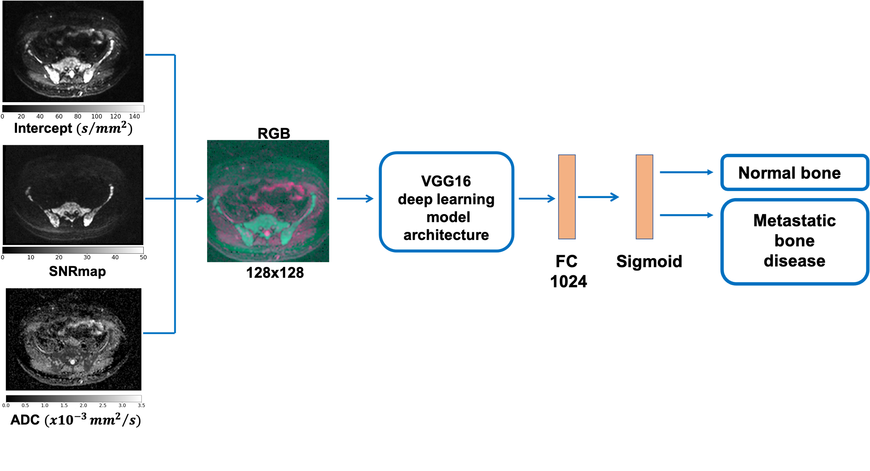
In this study, we used the pre-trained weights of the VGG16 model up to, but not including the final layer, which encoded input images as a 1024-length vector. The results were fed into a second fully connected network with 1024 input nodes and 2 output nodes (sigmoid activation), which was trained for detecting the presence of disease within slices [5] (Figure 1). Input images consisted of 3-channels (representing an RGB encoding, see Figure 1): (R) calculated the b=0 $$$\ s/mm^2$$$ image (the intercept from linear fitting of the DWI data) [6], (G) high b-value signal-to-noise-ratio map (SNRmap) to improve signal normalization between different WBDWI scans. SNRmap was calculated according to
$$S_{SNRmap} = S_{b900}/\sigma$$
where $$$S_{b900}$$$ is the image signal in the b=900 $$$s/mm^2$$$ images, and $$$\sigma$$$ is the standard deviation of $$$S_{b900}$$$ values within background voxels, and (B) the reconstructed ADC map. Images were interpolated to matrix=128x128 and resolution=2.5x2.5mm. All the images were scaled to ensure values were in the range [0, 1] using the following transformations:

$$$ADC \rightarrow ADC\ /\ 3.5 \times 10^{-3}mm^2/s$$$

$$$Intercept \rightarrow log(Intercept)\ / \ max(log(Intercept))$$$

$$$SNRmap \rightarrow log(SNRmap)\ / \ max(log(SNRmap))$$$

The ground truth was determined by an experienced radiologist who manually annotated normal/metastatic bone using WBDWI, T1-weigthed and Dixon imaging in all patient datasets.
Patient data were split into training, validation and test datasets; 31 patients were used for training/validation (7187 and 5528 axial images for normal and metastatic bone disease respectively) and 8 for testing. Adam optimisation (learning rate $$$10^{-3}$$$) was used to minimise a binary cross-entropy loss function over 80 epochs using a batch size of 256. All algorithms were implemented using Tensorflow 2.0 and Keras toolboxes.

Results

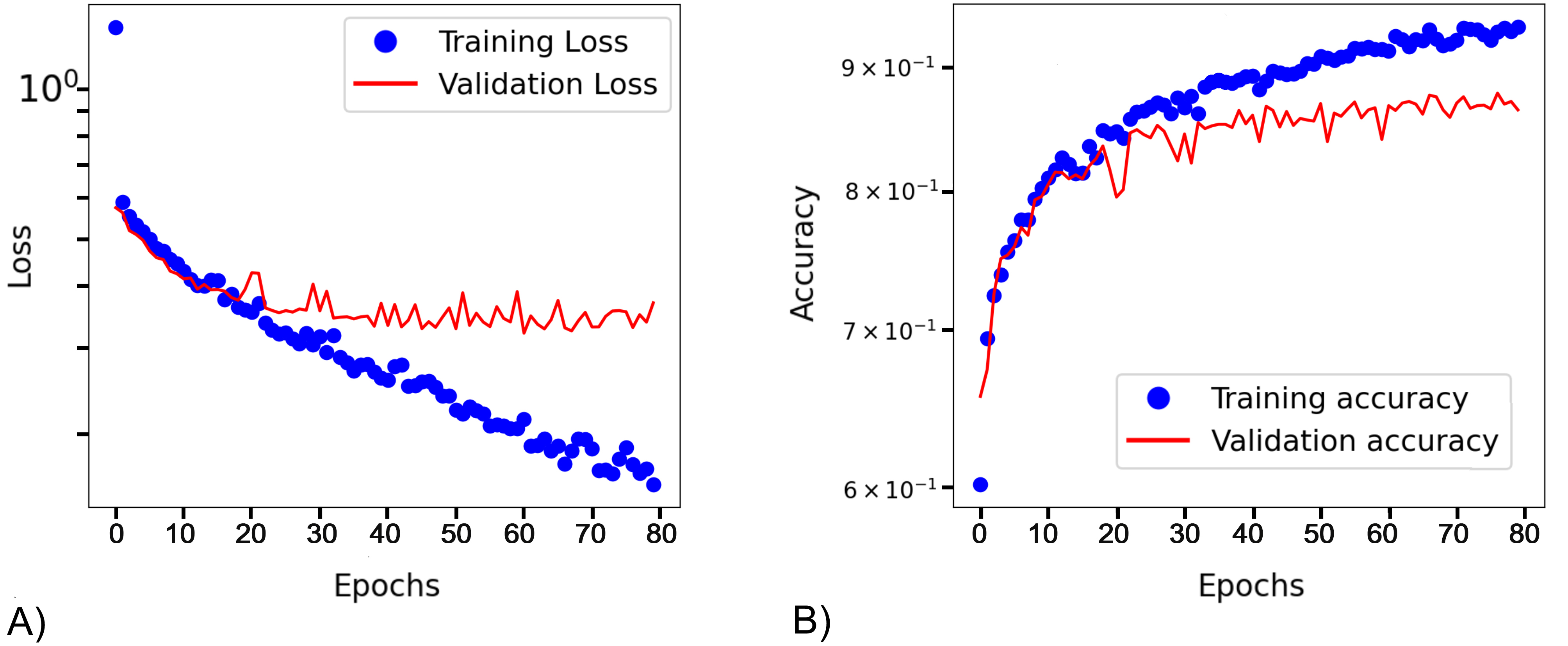
Figure 2 shows training and validation curves. After 40 epochs a plateau was observed with value for validation loss and accuracy of 0.25 and 0.85, respectively.
The model showed an accuracy of 0.88 (sensitivity/specificity of 0.87/0.89) on our test dataset using a cut-off value for the probability of presence of metastatic bone disease higher than 0.5.
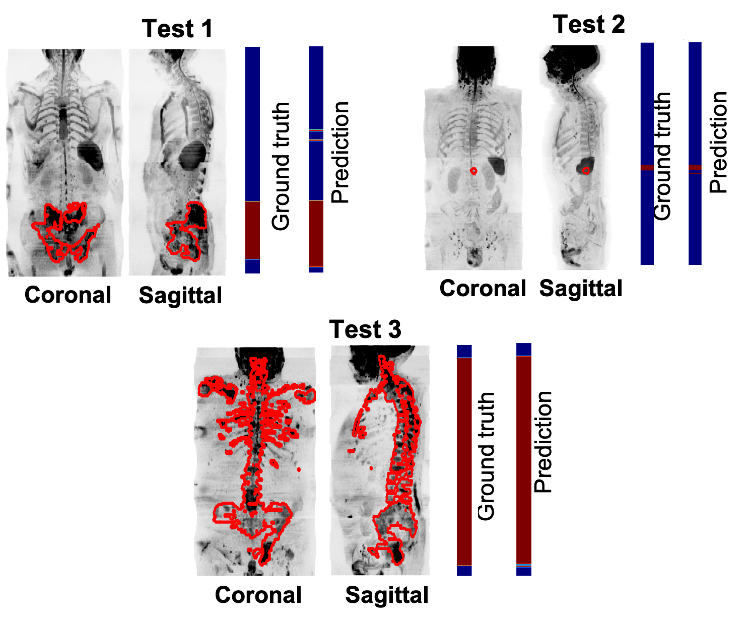
Figure 3 shows the prediction along the coronal and sagittal plane for 3 patients that belong to the test data. The number of axial images mis-classified was less than 5%.
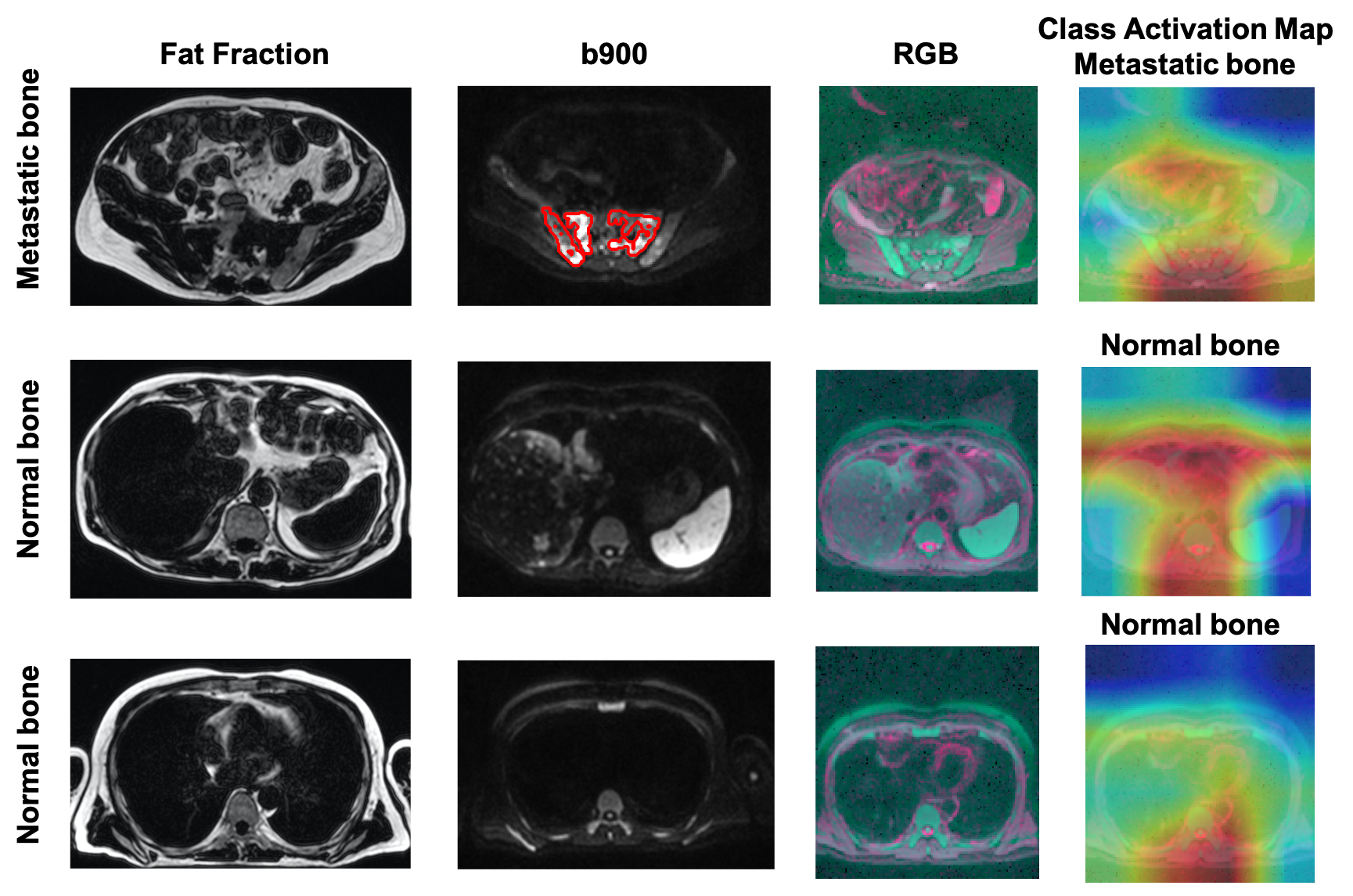
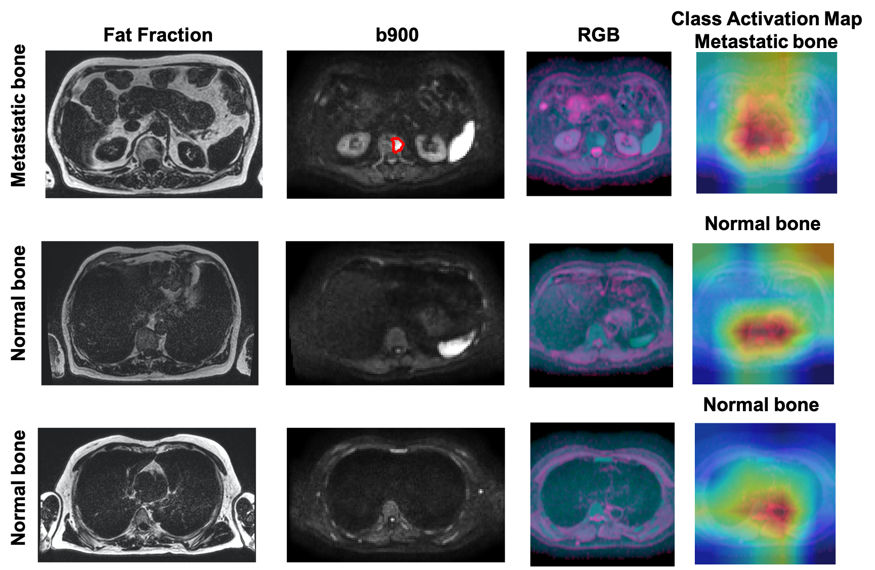
Figures 4 and 5 show the fat fraction, b900 and derived RGB images in the axial plane for two test patients. It should be noted that the model was able to successfully predict the absence/presence of bone disease in individual slice-locations with high accuracy.
To improve the explainability of the model, the class activation map (CAM) was derived [7]. CAM emphasizes important regions within the images that the model uses to make a particular decision. In this case, CAM shows that the relevant features are typically within the skeleton.

Discussion

The classification of metastatic bone disease in APC patients is not a trivial task. Radiologists may require different MRI modalities to detect presence of disease ‘at a glance’. Our transfer learning model shows promising results in classifying normal/metastatic bone on individual WBDWI slices, potentially accelerating diagnostic evaluation of these datasets without the requirement of Dixon imaging.

Acknowledgements

The authors would like to acknowledge Mint Medical®; Invention for Innovation, Advanced computer diagnostics for whole body magnetic resonance imaging to improve management of patients with metastatic bone cancer II-LA-0216-20007; and NIHR Clinical Research Facilities and Biomedical Research Centre at the Royal Marsden Hospital and Institute of Cancer Research.