Introduction

Quantification of myelin content in the white matter (WM) is essential for studying developmental processes and neurodegenerative diseases^1-3. Direct assessment of myelin, however, is highly impractical on clinical MRI scanners due to the limit on achievable resolutions. This limitation is circumvented by modeling WM T₂-signals as a weighted average over three tissue compartments: intra/extra-cellular water and myelin water⁴. This signal model can cast into a linear matrix form: $$S=Ew+H\ \ \ \small(1)$$where $$$S$$$ is the experimental signal comprised of time-points, $$$E$$$ is a simulated dictionary of single-T₂ signals expected in the tissue, $$$w$$$ is an unknown weights vector representing the relative fractions of the elements in $$$E$$$, and $$$H$$$ is an unknown noise vector. Such modeling allows to match each signal with a distribution of T₂ relaxation times (T₂-spectrum) and use the obtained spectrum to quantify the myelin water fraction (MWF) – a proxy of myelin content^2,5-6. Notwithstanding its advantages mcT₂ analysis faces major challenges, leading to a lack of a gold standard technique⁷. The key challenge, in this case, is the ambiguity, which arises due to the large number of possible T₂ combinations resulting in a highly ill-posed problem^8-10.
Recently, we introduced a new data-driven algorithm for mcT₂ analysis. Assuming the existence of only a finite number of microstructural compartmentations, the algorithm first applies statistical tests to identify a series of global mcT₂ features in the anatomy in question. It then uses these to analyze voxel-specific signals using a designated optimization scheme. Unlike spatially local approaches^8,11, the statistical power produced by this global approach endows the analysis with additional robustness, which stabilizes the localized optimization scheme. Preliminary validations of the algorithm’s accuracy were presented on two and three-compartment phantoms¹². We present here a complete version of the algorithm including validations on in vivo brain WM.

Methods

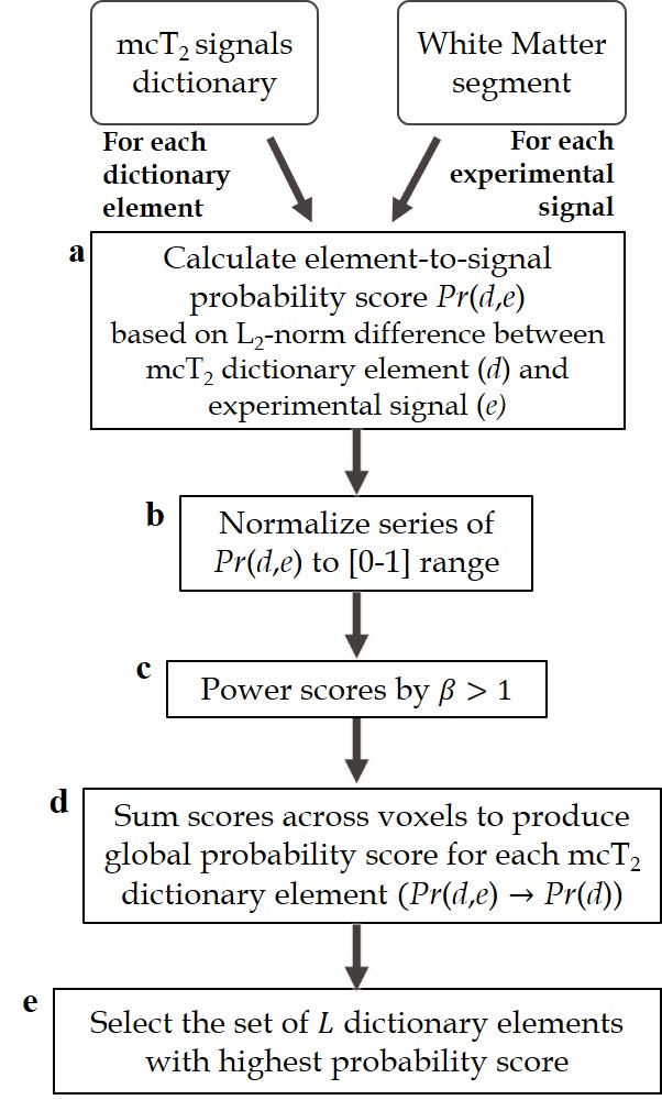
mcT₂ Algorithm
i. Generate a broad mcT₂ dictionary containing all possible combinations of multi-T₂ distributions by superimposing sets of simulated single-T₂ signals generated by the echo-modulation algorithm^13,14.

ii. Calculate the statistical correlation between dictionary elements ($$$d$$$) and experimental signals ($$$e$$$) in the anatomy in question ($$$\small\tt \color{navy} {Fig.1a}$$$). This provides a pairwise score $$$Pr(d,e)$$$, which is normalized to [0…1] ($$$\small\tt \color{navy} {Fig.1b}$$$) and subsequently raised to the power of $$$\beta$$$ to prioritize mcT₂ signals with higher statistical correlation ($$$\small\tt \color{navy} {Fig.1c}$$$).

iii. Sum the scores of each dictionary element across all voxels to form a global, element-specific, probability score $$$Pr(d) $$$ ($$$\small\tt \color{navy} {Fig.1d}$$$).
iv. Identify the set of $$$L$$$ dictionary elements with highest scores and denote them as $$$\widehat{E}$$$ ($$$\small\tt \color{navy} {Fig.1e}$$$). Then substitute the term $$$Ew$$$ in Eq. (1) and express the signal as a weighted sum of mcT₂ motifs. $$S= \widehat{E}\widehat{W}+H\ \ \ \small(2)$$ where $$$\widehat{W}$$$ is the unknown weights of each mcT₂ motif in $$$\widehat{E}$$$.

v. Cast Eq. (2) as the following minimization problem:$$argmin_{\widehat{W}}(\phi)=\frac{1}{2}||\widehat{E}\widehat{W}-S||_2^2+\lambda_{Tik}|\widehat{W}||_2^2+\lambda_{L1}|\widehat{W}||_1\ \ \ \ s.t.\ \widehat{W}_i\geq0,\ \sum\widehat{W_i}=1\ \ \ \small(3)$$ Here $$$\lambda_{Tik}$$$ and $$$\lambda_{L1}$$$ are Tikhonov and L₁ regularization weights. The inequality constraints ensure that is non-negative and forces its sum to be unity, as expected in case of T₂ spectrum.

vi. Solve Eq. (3) using MATLAB’s quadratic programming optimizer (Mathworks, Natick, Massachusetts, USA).

MRI scans
In vivo brain scans were performed on a 3 Tesla whole body MRI scanner (Prisma, Siemens Healthineers) using a 24-channel head coil. To test reproducibility, three identical multi-echo spin-echo scans were performed for the same subject, during one scan session. Experimental parameters were: FOV=200x210 mm², matrix size=216x180, N_averages=1, TR=3000 ms, TE=10, 20,...,200 (N_TE’s=15), slice thickness=3 mm, acquisition-bandwidth=210 Hz/Px.

mcT₂ analysis
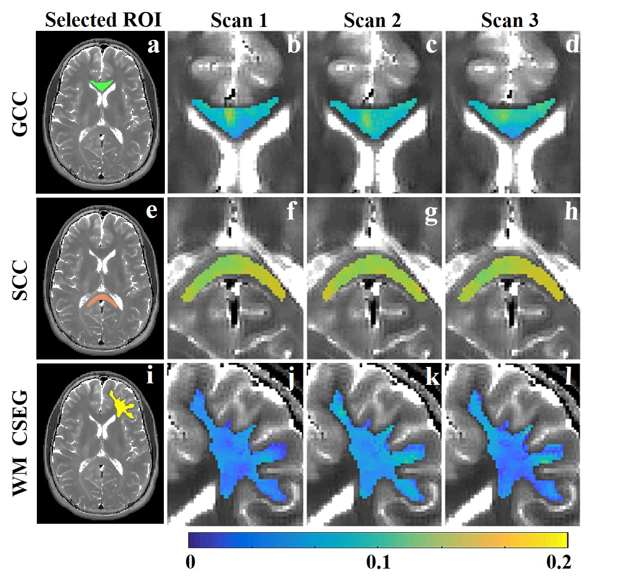
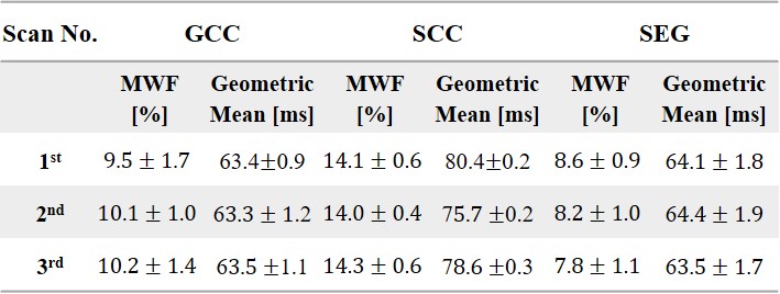
Three WM segments were investigated: the genu corpus callosum (GCC), splenium of corpus callosum (SCC) and a cortical segment (CSEG). Segments data were analyzed with a mcT₂ dictionary containing 64 elements, logarithmically spaced between 1-800 ms, and fraction resolution of 0.05 for T₂’s$$$\leq$$$40 ms and 0.1 for T₂’s$$$>$$$40. Spatially global statistical analysis was done using $$$\beta$$$=10⁴ and $$$L$$$=30 . Eq. (3) was solved using MATLAB’s solver with $$$\lambda_{Tik}$$$=10^-2 and $$$\lambda_{L1}$$$=10³. Mean and standard deviations (SD) of MWF values (T₂$$$\leq$$$40)² were calculated, along with the geometric mean of the remaining T₂-spectrum (T₂>40)¹⁵.

Results

$$$\small\tt \color{navy} {Fig.2}$$$ presents MWF maps of the three WM segments. MWF values for the CSEG and SCC ranged between 8-13% and 10-16% respectively, while the GCC values ranged between 5-14%. Segment specific mean and SD of MWF values are delineated in $$$\small\tt \color{navy} {Table\ 1}$$$. These values demonstrate a consistent range of MWF values with similar means and relatively low SDs of 1.4% (GCC), 0.5% (SCC), and 1.0% (CSEG), across scans. The geometric means and SDs were also consistent between scans ($$$\small\tt \color{navy} {Table\ 1}$$$).

Discussion & Conclusion

This study presents the first use of global mcT₂ analysis approach on clinical data. Our results show that the proposed method can reproducibly probe MWF in the WM tissue at in vivo scan settings and, thereby allowing to track microscopic myelin-related processes. The results further demonstrate that learning global tissue features prior to performing voxel-based mcT₂ analysis stabilizes the optimization scheme and efficiently overcomes the ambiguity in the T₂-space without the need to assume the number of sub-voxel tissue compartments.

References

1.Heath F, Hurley A, et al. Advances in noninvasive myelin imaging. Dev. Neurobiol. 2018;78:136–151.
2. Alonso-Ortiz E, Levesque R, et al. MRI-based myelin water imaging: A technical review. Magn. Reson. Med. 2015;73(1):70-81.
3. Möller E, et al. Iron , Myelin , and the Brain : Neuroimaging Meets Neurobiology. Trends Neurosci. 2019;42(6):384-401.
4. Lancaster J, et al. Three-pool model of white matter. J. Magn. Reson. Imaging. 2003;17:1-10.
5. Mackay A, et al. In vivo visualization of myelin water in brain by magnetic resonance. Magn. Reson. Med. 1994;31(6):673-677.
6. Laule C, et al. Myelin water imaging of multiple sclerosis at 7 T: Correlations with histopathology. Neuroimage. 2008;40(4):1575-1580.
7. Does M. Inferring brain tissue composition and microstructure via MR relaxometry. NeuroImage. 2018;182(136-148).
8. Whittall P and MacKay L. Quantitative interpretation of NMR relaxation data. J. Magn. Reson. 1989;84:134-152.
9. Graham S, et al. Criteria for analysis of multicomponent tissue T2 relaxation data. Magn. Reson. Med. 1996;35:370–378.
10. Laule C, et al. Water content and myelin water fraction in multiple sclerosis - a T2 relaxation study. J. Neurol. 2004;251:284–293.
11. Whittall K. Recovering compartment sizes from NMR relaxation data. J. Magn. Reson. 1991;94(3):486-492.
12. Omer N, et al. A novel multicomponent T2 analysis for identification of sub-voxel compartments and quantification of myelin water fraction. E-poster, 28th Proc Intl Soc Mag Reson Med, p. 6109, online (2020).
13. Ben-eliezer N, Sodickson D K, et al. Rapid and Accurate T2 Mapping from Multi–Spin-Echo Data Using Bloch-Simulation-Based Reconstruction. 2015;73(2):809-817.
14. Hennig J. Multiecho imaging sequences with low refocusing flip angles. J Magn Reson 1988;78:397–407.
15. Whittall K, et al. In vivo measurement of T2 distributions and water contents in normal human brain. Magn. Reson. Med. 1997;37(1):34–43.