Introduction

Diffusion-weighted MRI (DWI) is used widely in the clinic. However, its biological interpretation remains an area of active investigation. Recently, a DWI simulation library based on three metabolic and cytometric tissue parameters (homeostatic cellular water efflux rate constant [k_io], cell density [ρ], and mean cell volume [V]), has been suggested and tested using Monte Carlo random walks within Voronoi-cell ensembles.^1,2 Using aMRI library-simulated DWI data that matches experimental pancreatic DWI results, the goal of this work is to investigate the optimal b-value sampling strategy for accurate parameter extraction under the constant data-acquisition time (fixed number of b-values) condition.

Methods

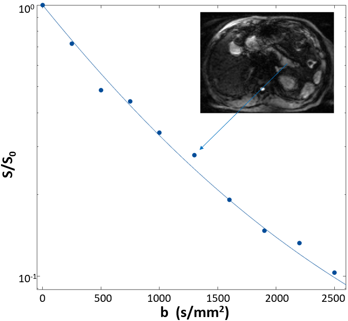
After informed consent, DWIs were acquired on normal subjects. The protocol employed thirteen b-values with 128x128 in-plane matrix, (36 cm)² FOV, and 5.0 mm slice thickness for a total acquisition time of ~4.7 minutes. The DWI decays were first de-noised^3,4 before applying library-matching to obtain the best-matched parameter set. Figure 1 shows a de-noised single-voxel DWI curve from the pancreatic tail. The inset shows the b = 750 s/mm² DW image. The blue best-matching curve and its parameter values [k_io = 71 s^-1, ρ = 660,000 cells/μL, V = 1.1 pL] were then taken as “true” inputs for acquisition optimization simulations.
To make the simulation closer to clinical protocols, we investigate the optimal acquisition under seven b-values (constant acquisition time). The optimal b-value extent (maximum) and distribution is investigated through Monte Carlo simulations. The primary b-value spacing employed a power‑law sampling pattern⁵ defined as: b_i = b₁ + (b_n - b₁) · [(i - 1) / (n - 1)]^r where b₁ and b_n are the first and last b values; n is the total number [here, 7]; b_i is the i^th value [the index i runs from 1 to n]; the exponent r determines the b value spacing. Additional b spacing included common logarithmic strategies. The b_n value, b_max, was varied from 2,000 to 7,000 s/mm² for all sampling patterns.
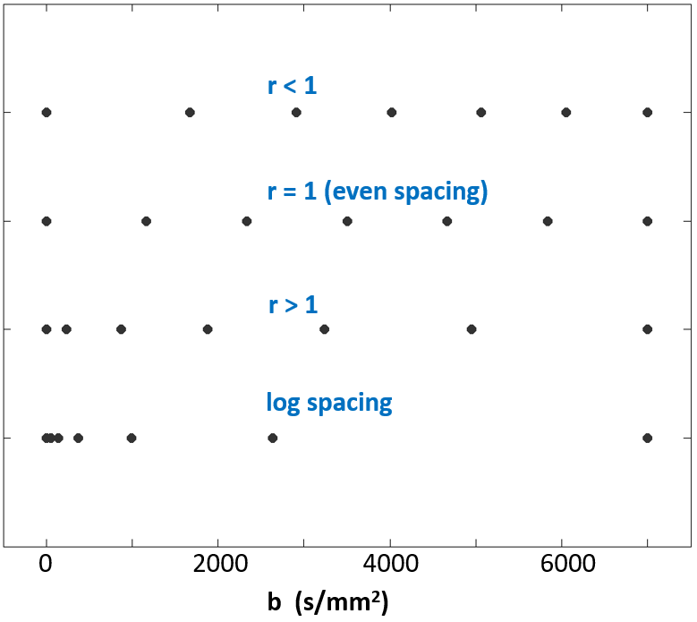
Representative spacings, with b_max = 7,000 s/mm², are shown in Figure 2. When r < 1, spacing is larger at lower b values (i.e., sampling weighted more towards high b); when r = 1, there is even sampling; when r > 1, spacing is larger at higher b values (i.e., sampling weighted more towards initial DWI decay). The log-spacing shown at the bottom represents a different sampling strategy heavily sampled at lower b-values. For each b‑array, 2,500 simulations were run with Rician signal distribution⁶ produced by adding random Gaussian noise to both real and imaginary channels independently before sum-of-square signal reconstruction. Each individual set of 2,500 simulations created at different signal‑to-noise ratios (SNRs) is then reshaped to a 50x50 matrix, and the same de-noising method^3,4 was applied to the simulated data. After de-noising, no appreciable deviation from Gaussian signal distribution was observed in any 2,500 samples.
Since the library approach lacks analytical methods for defining a standard error surface in a multi-variate problem, matching accuracy (a), defined as the fraction (a ≤ 1) of the matched de-noised curves returning all three parameters correctly, is used to evaluate the performance of individual sampling pattern. Matching error is then (1.0 – a), whose natural log value is generally negative.

Results

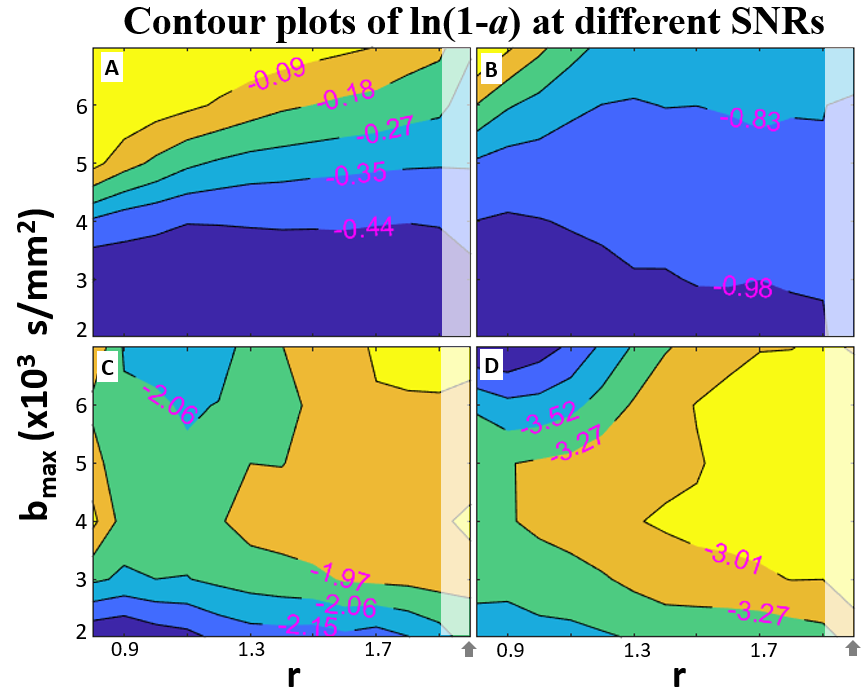
Figure 3 shows contour plots of ln(1.0 – a) for simulations with different b_max (from 2,000 to 7,000) values and different b-spacing power (r) values at four different single channel (real or imaginary) SNR (at b = 0) values: 50 (A), 100 (B), 200 (C), 300 (D). ln(1.0 – a) contours are used to mimic the common appearance of error surfaces, where the lowest [i.e., most negative (bluer)] value represents preferred outcome. For the healthy pancreatic tail, b_max under 3,000 s/mm² is sufficient for practical achievable SNR (~50-100) and b-spacing pattern is often not critical for these SNRs. Only when SNR ≥ 300, does it become possible to see the benefit of high b_max (D). Overall, the even-spaced b-value array (r = 1) remains a good option.

Discussion

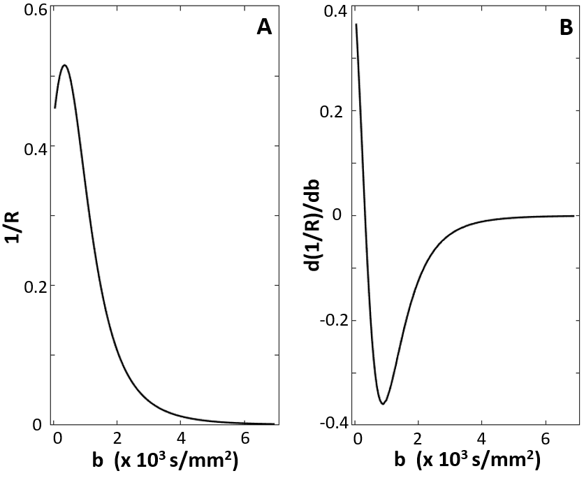
Under a constant acquisition-time constraint, the optimal DWI data acquisition strategy for the pancreatic tail is shown to be an even-spaced b-array with a maximum b-value under ~3,000 s/mm². With an up-sampled b-array, Figure 4 provides some additional insights. In 4A, the numerically determined radius (R) of curvature reciprocal for the “true” DWI curve (Fig. 1 solid curve) is plotted against the b‑values. When 1/R approaches zero, the b-space decay approaches straight line. Fig. 4B plots the derivative of (1/R) with respect to b-values. This quantifies how quickly the curvature changes. It is obvious the most dramatic changes occur when b < 3,000 s/mm² for normal pancreatic tail, matching the Fig. 3 simulation results. It is worth noting that the current optimized strategy should work for pancreatic head and body as well, as observed diffusivity is similar in the entire pancreas.⁷ It is expected that different tissue types with different DWI decay patterns will have different optimal strategies. For example, a prostate lesion has a significantly lower diffusivity, and the Fig. 4B analogy remains significantly non-zero for b-values over 4,000 s/mm². For this, an r > 1 and b_max > 4,000 can be a preferred strategy (data not shown).

References

1. Baker, Moloney, Li, Gilbert, Springer, PISMRM, 28:3612 (2019).
2. Baker, Moloney, Li, Wilson, Barbara, Maki, Gilbert, Springer, PISMRM, 28:3585 (2019).
3. Veraart J, Novikov DS, Christiaens D, Ades-Aron B, Sijbers J, Fieremans E. Neuroimage. 142:394-406 (2016).
4. Does, Olesen, Harkins, Serradas-Duarte, Gochberg, Jespersen, Shemesh. Magn Reson Med. 81:3503-3514 (2019).
5. Reci, Ainte, Sederman, Mantle, Gladden, MRI, 56:14-18 (2019).
6. Cardenas-Blanco, Tejos, Irarrazaval, Cameron. Concepts Magn Reson Part A 32A:409 – 416 (2008).
7. Barral, Taouli, Guiu, Koh, Luciani, Manfredi, Vilgrain, Hoeffel, Kanematsu, Soyer. Radiology. 274:45-63 (2015).