3642
Computing the Orientational-Average of Diffusion-Weighted MRI Signals: A Comparison of Different Techniques1Cardiff University Brain Research Imaging Centre (CUBRIC), School of Psychology, Cardiff University, Cardiff, United Kingdom, 2Department of Biomedical Engineering, Linköping University, Linköping, Sweden, 3Center for Medical Image Science and Visualization, Linköping University, Linköping, Sweden, 4These authors share last authorship, Linköping, Sweden, 5These authors share last authorship, Cardiff, United Kingdom
Synopsis
Numerous applications in diffusion MRI involve computing the orientationally-averaged diffusion-weighted signal. Most approaches assume that the gradient vectors are uniformly distributed on a sphere, computing the orientationally-averaged signal through arithmetic averaging. One challenge is that not all acquisition schemes have gradient vectors distributed over perfect spheres. Alternative averaging methods include: weighted signal averaging; spherical harmonic; and Mean Apparent Propagator MRI (MAP-MRI). Here, these methods are compared under different signal-to-noise (SNR) realizations. With dense and isotropically-distributed sampling, all methods give comparable results. As the SNR and number of data points are reduced, MAP-MRI-based approaches give pronounced improvements over the other methods.
INTRODUCTION
Diffusion MRI is a non-invasive technique that is sensitive to differences in tissue microstructure. Due to the emerging interest 1-10 in employing the ``powder-averaged signal'', 11-13 we consider the problem of estimating this quantity. The accuracy of the powder-averaged signal depends on both the set of gradient directions and the numerical method used to estimate the average. Regarding the former, the most well-known approach is the electrostatic repulsion algorithm.14-16 In some applications, the sample points should be optimally distributed across three-dimensional $$$q$$$-space. 17,18 The second important factor is the method used to compute the powder-average. Methods that perform brute-force estimation of the signal average 19,20 as well as those that take the ``isotropic component'' of the signal, 12,21-22 are compared.THEORY
1. Arithmetic averagingThe simplest technique for powder-averaging is the arithmetic mean. 20
$$\bar{S}=\frac{1}{n_\mathrm{dir}}\sum_{i=1}^{n_\mathrm{dir}}S_i\quad\quad(1)$$
where $$$\bar{S},\,n_\mathrm{dir}$$$, and $$$S_i$$$ are, respectively, the orientationally-averaged signal, number of gradient directions, and the signal along the $$$i$$$th direction.
2. Weighted averaging
Weighted averaging can be used to account for the non-uniformity of the gradient directions. 23,24
$$\bar{S}=\frac{\sum_{i=1}^{n_\mathrm{dir}}w_i\, S_i}{\sum_{i=1}^{n_\mathrm{dir}}\,w_i}\quad\quad(2)$$
where $$$w_i$$$ are the weights.
2.1 Quadratures on the sphere (Lebedev)
Lebedev quadrature evaluates integrals over the unit sphere,
$$I=\int_0^{2\pi}\int_0^\pi\,f(\theta,\phi)\,\sin\theta\,\mathrm{d}\theta\,\mathrm{d}\phi\quad\quad(3)$$
$$I\approx\sum_{i=1}^N\,f(\theta_i,\phi_i)\,w_i\equiv\,Q[f]\quad\quad(4)$$
where the points ($$$\theta_i,\,\phi_i$$$) and weights $$$w_i$$$ are estimated for different $$$N$$$ using the algorithm in 25. $$$Q[f]$$$ is the quadrature of the exact integral.
2.2 Representation of the single-shell signal in a series of spherical harmonics (SH)
Any square-integrable function, $$$F(\hat{\mathbf{x}})$$$, can be represented as:
$$F(\hat{\mathbf{x}})=\sum_{k=0}^\infty\sum_{m=-k}^k f_{km}\,Y_k^m (\hat{\mathbf{x}})\quad\quad(5)$$
where $$$k$$$ and $$$m$$$ indicate the order of the SH function ($$$Y_k^m(\hat{\mathbf{x}})$$$). The coefficients are:
$$f_{km}=\int\,F(\hat{\mathbf{x}})\,Y_k^m(\hat{\mathbf{x}})^*\,\mathrm\,d\hat{\mathbf{x}}\quad\quad(6)$$
If $$$F(\hat{\mathbf{x}})$$$ is rotationally-invariant, all coefficients except $$$f_{00}$$$ vanish. 26
$$\mathbf{s}=\mathbf{Ya}\quad\quad(7)$$
where
$$$\mathbf{s}_{n_\mathrm{dir}\times\,1},\,\mathbf{Y}_{n_\mathrm{dir}\times\,n_\mathrm{coeff}}\,n_\mathrm{coeff}=(L+1)(L+2)/2$$$, and $$$\mathbf{a}_{n_\mathrm{coeff \times\,1}}$$$ are the diffusion-weighted signals, matrix of SHs, number, and the vector of coefficients 12
$$\mathbf{a}=(\mathbf{Y}^\intercal\mathbf{Y})^{-1}\mathbf{Y}^\intercal\mathbf{s}\quad\quad(8)$$
$$\bar{S}=a_0\,Y_0^0=a_0/\sqrt{4\pi}\quad\quad(9)$$
($$$Y_0^0=1/\sqrt{4\pi}$$$ 27).
2.3 Representation of the single-shell signal using Cartesian tensors
The diffusion-weighted signal can also be represented as:
$$S(\mathbf{\hat{u}})=\mathbf{\hat{u}}^\intercal\mathbf{M}\mathbf{\hat{u}}\quad\quad(10)$$
where $$$\mathbf{\hat{u}}$$$ is the gradient direction and $$$\mathbf{M}_{3\times3}$$$ is a symmetric positive definite matrix. 28,29
$$\bar{S}=\mathrm{Tr}(\mathbf M)/3\quad\quad(11)$$
2.4 Knutsson approach
Consider a weighted sampling function of the form
$$G(\hat{\mathbf{x}})=\sum_{i=1}^{n_\mathrm{dir}} w_i\,\delta(\hat{\mathbf{x}}-\hat{\mathbf{u}}_i)\quad\quad(12)$$
The coefficients of this function in the SH basis are:
$$g_{km}=\sum_{i=1}^{n_\mathrm{dir}}w_i\,Y_k^m(\hat{\mathbf{u}}_i)^*\quad\quad(13)$$
So we have:
$$$g_{km}\propto\delta_{k0}\delta_{m0}$$$.
$$$\mathbf{g}_0$$$ is the vector of coefficients having non-zero value when $$$k=m=0$$$. An optimal vector of weights, $$$\mathbf{w}_0$$$, is 23:
$$\mathbf{w}_0=\mathrm{argmin}[(\mathbf{Bw}-\mathbf{g}_0)^\intercal\mathbf{V}(\mathbf{Bw}-\mathbf{g}_0)]=(\mathbf{B}^\intercal\mathbf{VB})^{-1}(\mathbf{VB})^\intercal\mathbf{g}_0\quad\quad(14)$$
where $$$\mathbf{B}$$$ and $$$\hat{\mathbf{u}}_i$$$ are, respectively, the matrix of the SH basis and the weights. 23 $$$\mathbf{V}$$$ is a diagonal matrix with elements $$$(1+k^2/36)^{-1}$$$.
3. MAP-MRI
The formulation of MAP-MRI is (equation (58) in 22):
$$S(q,\mathbf{\hat q})=\sum_{N=0}^{N_\mathrm{max}}\sum_{j,l}\sum_{m=-l}^{l}\kappa_{jlm}\Xi_{jlm}(u_0,q,\mathbf{\hat q})\quad\quad(15)$$
where $$$j\geq1,\,l\geq0$$$ and $$$2j+l=N+2$$$, $$$u_0$$$ is a scalar, and $$$q$$$ and $$$\mathbf{\hat{q}}$$$ are the magnitude and direction of the wavevector and:
$$\Xi_{jlm}(u_0,q,\mathbf{\hat q})=\sqrt{4\pi}i^{-1}(2\pi^2u_0^2q^2)^{l/2}e^{-2\pi^2u_0^2q^2}L_{j-1}^{l+1/2}(4\pi^2u_0^2q^2)Y_{l}^m(\mathbf{\hat{q}})\quad\quad(16)$$
where $$$L_{k}^{\alpha}(.)$$$ is the associated Laguerre polynomial.
The powder-averaged signal is obtained by setting $$$l=m=0$$$ and $$$j=1+N/2$$$:
$$\bar{S}=\sum_{N=0}^{N_\mathrm{max}}\kappa_{(1+N/2)00}\,\Xi_{(1+N/2)00}(u_0,\mathbf{q})\quad\quad(17)$$
MATERIALS AND METHODS
The noise-free diffusion-weighted signal is:$$S(b,\mathbf{\hat{u}})=\int W(\mathbf{\hat n})\,e^{-b\mathbf{\hat u}^\intercal\,\mathbf{D}(\mathbf{\hat n})\,\mathbf{\hat{u}}}\,\mathrm{d}\mathbf{\hat{n}}\quad\quad(18)$$
where $$$\mathbf{D}(\mathbf{\hat{n}})$$$ is an axisymmetric tensor ($$$\mathbf{\hat n}=(0.4,\,0.6,\,-0.693)^\intercal$$$, $$$D^{\mid\mid}=1$$$, and $$$D^{\perp}=0.14\,\mu m^2/ms$$$) and $$$W(\mathbf{\hat{n}})$$$ is Watson orientation distribution function (ODF) with $$$\kappa=$$$1, 9, and $$$\infty$$$).
The ground truth (gt) value is 6,30:
$$\bar{S}_\mathrm{gt}(b)=\frac{\sqrt{\pi }{e}^{-bD^{\perp}}}{2}\frac{\mathrm{erf}(\sqrt{b(D^{\mid\mid}-D^{\perp})})}{\sqrt{b(D^{\mid\mid}-D^{\perp})}}\quad\quad(19)$$
The data were computed at $$$b=0,\,1.5,\,3,\,4.5,\,6,\,7.5,\,9,\,10.5$$$, and $$$12\,ms/\mu m^2$$$ ($$$\Delta=43.1,\,\delta=10.6\,ms$$$, and $$$b=q^2(\Delta-\delta/3)$$$), therefore, $$$\bar{E}(b)=1,\,0.5640,\,0.3541,\,0.2386,\,0.1682,\,0.1221,\,0.0903,\,0.0678,\,0.0514$$$. The noisy signal values for Gaussian and Rician distributions, are:
$$S_\mathrm{ng}=\bar{S}_\mathrm{gt}+N_\mathrm{r}(0,\sigma_\mathrm{g})\quad\quad(20)$$
$$S_\mathrm{nr}=\sqrt{(\bar{S}_\mathrm{gt}+N_\mathrm{r}(0,\sigma_\mathrm{g}))^2+N_i(0,\sigma_\mathrm{g})^2}\quad\quad(21)$$
where $$$N_r(0,\sigma_\mathrm{g})$$$ and $$$N_i(0,\sigma_\mathrm{g})$$$ are the noise in the real and imaginary images ($$$\sigma_\mathrm{g}=0.1414,\,0.0707,\,0.0283,\,0.0071,\,0.0014$$$).
We utilized $$$d_1$$$ and $$$d_2$$$ for evaluation:
$$d_1=\frac{1}{24}\sum_{j=1}^8\sum_{k=1}^3|\bar S_\mathrm{est}(b_j,\kappa_k)-\bar{S}_\mathrm{gt}(b_j)|\quad\quad(22)$$
$$\epsilon_j=\frac{1}{3}\sum_{k=1}^3\bar{S}_\mathrm{est}(b_j,\kappa_k)-\bar{S}_\mathrm{gt}(b_j)\quad\quad(23)$$
$$d_2=\textrm{Pearson's correlation coefficient}(b_j,\epsilon_j)\quad\quad(24)$$
where $$$\bar{S}_\mathrm{est}$$$ and $$$\bar{S}_\mathrm{gt}$$$ are, the estimated and the ground truth values.
The gradient vectors were generated for $$$488,\,344$$$, and $$$152$$$ non-shelled and 61, 18 43 and 19 shelled point sets. 25
RESULTS
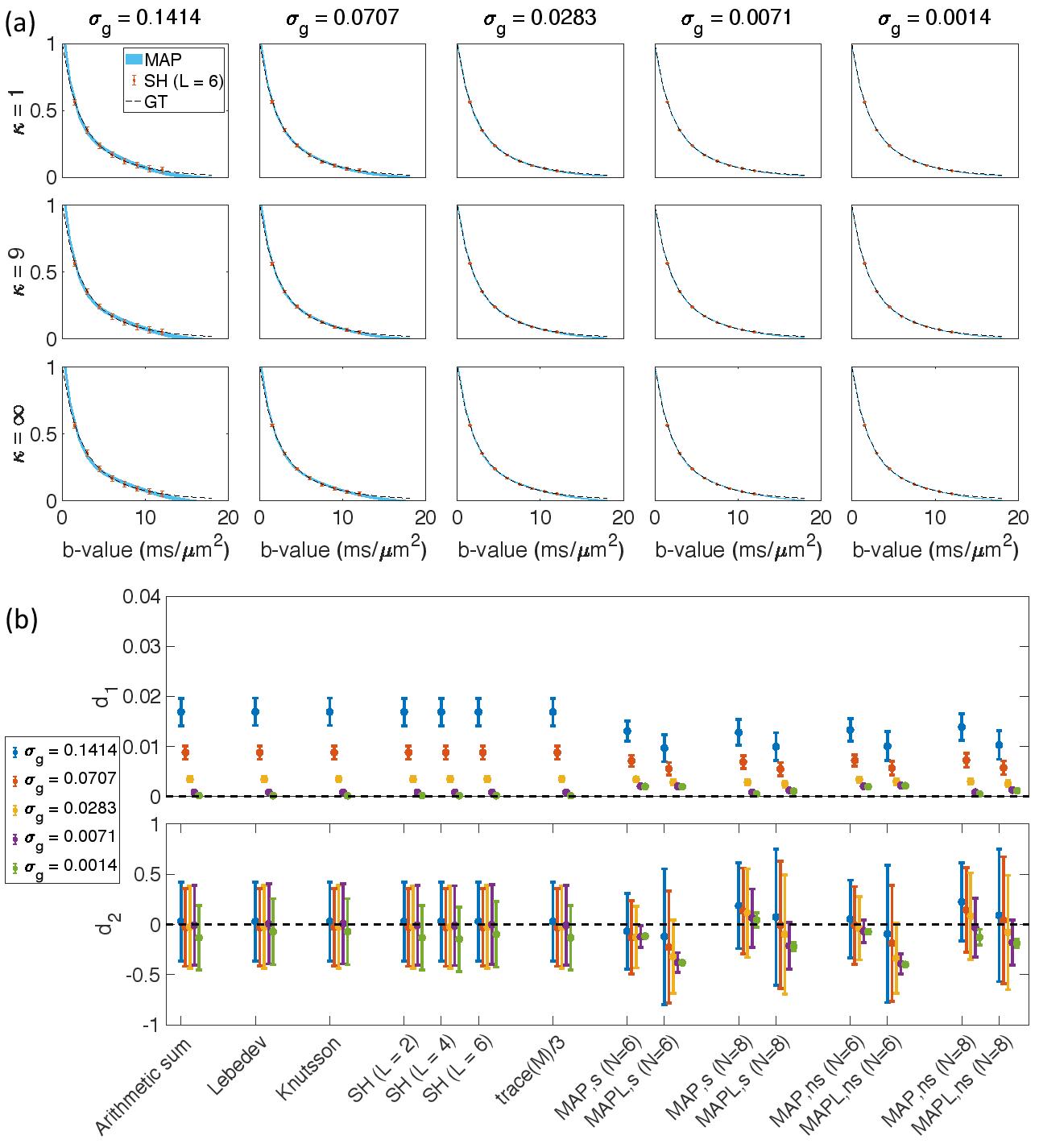
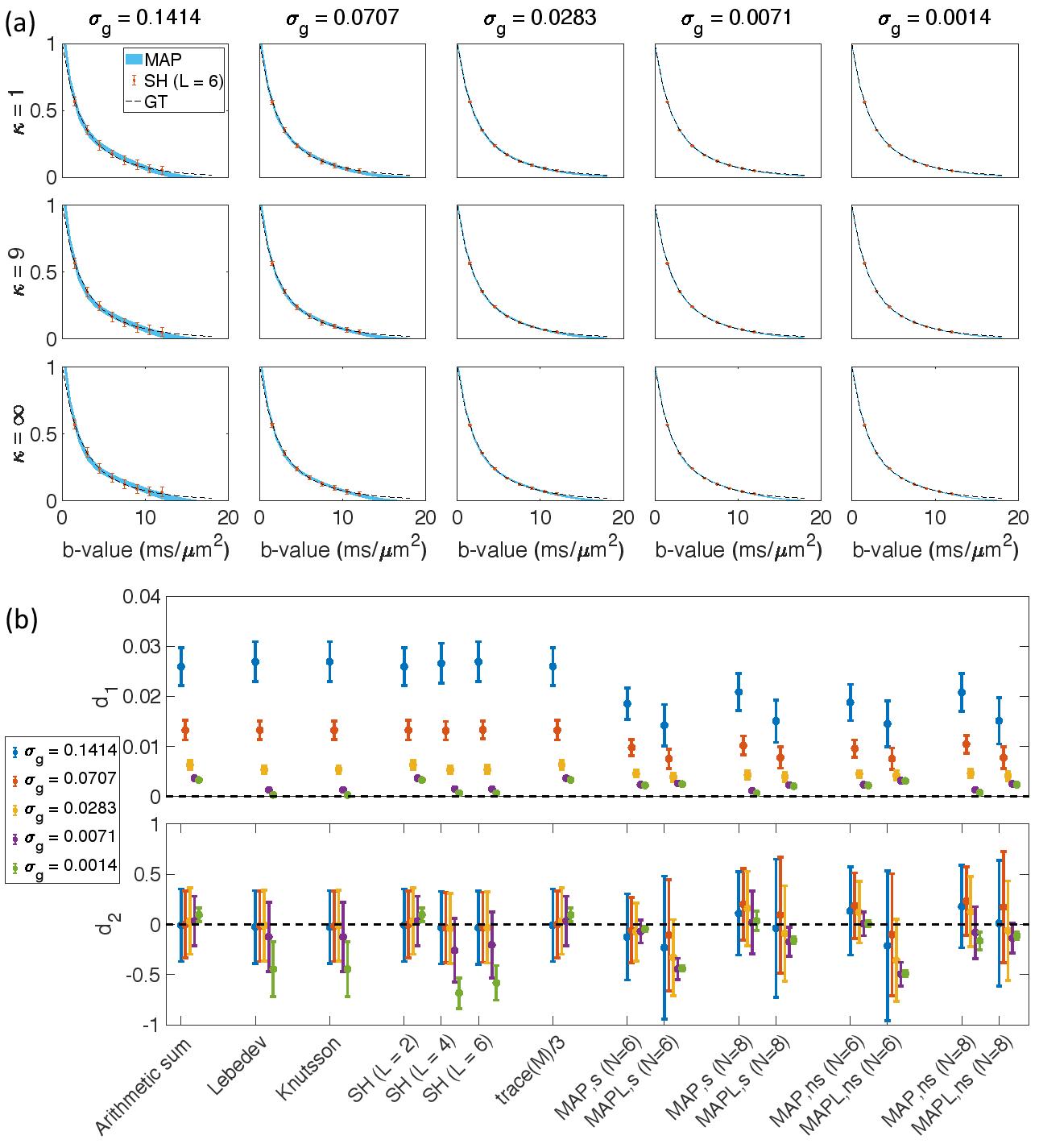
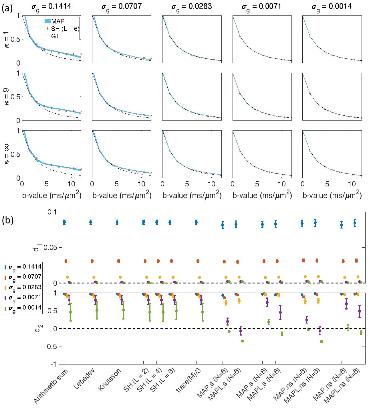
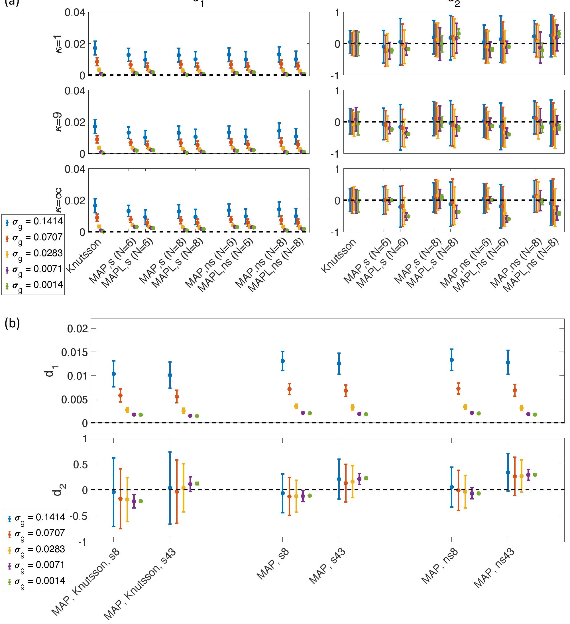
Fig. $$$1,\,2$$$, and $$$3$$$ illustrate the results obtained from $$$488,\,344$$$, and $$$152$$$ samples for both shelled ($$$61\times8,\,43\times8$$$, and $$$19\times8$$$) and non-shelled point sets with Gaussian noise. Fig. 4 shows the results obtained from the 344 ($$$43\times8$$$) sample scenario for Rician signal. MAPL 31 is regularized version of MAP.In Fig. 5(a), we assessed the effect of dispersion.
Fig. 5(b) illustrates the results of MAP-based interpolation. We used both shelled ($$$43\times8$$$) and non-shelled 344 point sets. `s8' and `s43' refer to the shelled point sets with 8, and 43 b-values, respectively.
To generate the `MAP,Knutsson,s8' and `MAP,Knutsson,s43', first, the signal was orientationally-averaged using the Knutsson method 23 at $$$b=1.5,\,3,\,4.5,\,\ldots,\,12\,ms/\mu m^2$$$, then the averaged signal was used to estimate the MAP-MRI coefficients and reconstruct the signal at $$$b=1.5,\,3,\,4.5,\,\ldots,\,12\,ms/\mu m^2$$$ (`MAP,Knutsson,s8') and $$$b=1.5,\,1.75,\,2,\,\ldots,\,12\,ms/\mu m^2$$$ (`MAP,Knutsson,s43'). The results `MAP,s8', `MAP,s43', `MAP,ns8' and `MAP,ns43' were obtained from the original data without averaging.
DISCUSSION AND CONCLUSION
Among the methods that can be performed on a shell-by-shell basis, the Lebedev quadrature 25 and Knutsson's approach 23,24 both show improved accuracy compared to arithmetic averaging approach, especially when there is a low number of point sets and SNR. Our simulations show that without correcting for Rician noise, the powder-averaged signal is far from the ground truth especially when SNR is low. As gradient strengths are pushed higher 32,33 maintaining gradient linearity becomes challenging 34. MAP-MRI is particularly well-suited to this situation. The MAPL 31 technique, is preferred over the original MAP only when bias with b-values is not a concern. The recent formulation 35 of the MAP method (MAP+) could improve the accuracy of the estimates.Acknowledgements
MA and DKJ are supported by a Wellcome Trust Investigator Award (096646/Z/11/Z) and DKJ by a Wellcome Trust Strategic Award (104943/Z/14/Z).This project was financially supported by the Swedish Foundation for Strategic Research (AM13-0090 and Multimodal Guidance in Neurosurgery), the Swedish Research Council 2015-05356 and 2016-04482, Linköping University Center for Industrial Information Technology (CENIIT), LiU Cancer, VINNOVA/ITEA3 17021 IMPACT, and Analytic Imaging Diagnostic Arena (AIDA).References
1. Lasiˇc, S., Szczepankiewicz, F., Eriksson, S., Nilsson, M. & Topgaard, D. Microanisotropy imaging: quantification of microscopic diffusion anisotropy and orientational order parameter by diffusion MRI with magic-angle spinning of the q-vector. Front. Phys.2, 11 (2014).
2. Szczepankiewicz, F.et al. Quantification of microscopic diffusion anisotropy disentangles effects of orientation dispersion from microstructure: applications in healthy volunteers and in brain tumors. NeuroImage104, 241–252 (2015).
3. Lawrenz, M. & Finsterbusch, J. Mapping measures of microscopic diffusion anisotropy in human brain white matter in vivo with double-wave-vector diffusion-weighted imaging. Magn. resonance medicine73, 773–783 (2015).
4. McKinnon, E. T., Jensen, J. H., Glenn, G. R. & Helpern, J. A. Dependence on b-value of the direction-averaged diffusion-weighted imaging signal in brain. Magn. resonance imaging36, 121–127 (2017).
5. Özarslan, E., Yolcu, C., Herberthson, M., Knutsson, H. & Westin, C.-F. Influence of the size and curvedness of neural projections on the orientationally averaged diffusion MR signal. Front. physics6, 17 (2018).
6. Herberthson, M., Yolcu, C., Knutsson, H., Westin, C.-F. & Özarslan, E. Orientationally-averaged diffusion-attenuated magnetic resonance signal for locally-anisotropic diffusion. Sci. reports9, 1–12 (2019).
7. Afzali, M., Aja-Fernández, S. & Jones, D. K. Direction-averaged diffusion-weighted MRI signal using different axisymmetric B-tensor encoding schemes. Magn. Reson. Medicine(2020).
8. Yolcu, C., Herberthson, M., Westin, C.-F. & Özarslan, E. Magnetic resonance assessment of effective confinement anisotropy with orientationally-averaged single and double diffusion encoding. arXiv preprint arXiv:1912.12760(2019).
9. Cheng, H., Newman, S., Afzali, M., Fadnavis, S. S. & Garyfallidis, E. Segmentation of the brain using direction-averaged signal of DWI images. Magn. Reson. Imaging69, 1–7 (2020).
10. Afzali, M.et al.Improving neural soma imaging using the power spectrum of the free gradient waveforms. InProc. Intl. Soc. Mag. Reson. Med. (2020).
11. Mitra, P. P. & Sen, P. N. Effects of microgeometry and surface relaxation on NMR pulsed-field-gradient experiments: Simple pore geometries. Phys Rev B45, 143–156 (1992).
12. Özarslan, E. & Basser, P. J. Microscopic anisotropy revealed by NMR double pulsed field gradient experiments with arbitrary timing parameters. The J. chemical physics128, 04B615 (2008).
13. Edén, M. Computer simulations in solid-state NMR. III. Powder averaging. Concepts Magn. Reson. Part A: An Educ. J.18, 24–55 (2003).
14. Jones, D. K., Horsfield, M. A. & Simmons, A. Optimal strategies for measuring diffusion in anisotropic systems by magnetic resonance imaging. Magn. Reson. Medicine: An Off. J. Int. Soc. for Magn. Reson. Medicine 42, 515–525 (1999).
15. Jones, D. When is a DT-MRI sampling scheme truly isotropic? In Proc Intl Soc Mag Reson Med, vol. 11, 2118 (2003).
16. Jones, D. K. Diffusion MRI (Oxford University Press, 2010).
17. Koay, C. G., Özarslan, E., Johnson, K. M. & Meyer and, M. E. Sparse and optimal acquisition design for diffusion MRI and beyond. Med Phys 39, 2499–2511, DOI: 10.1118/1.3700166 (2012).
18. Knutsson, H. Towards optimal sampling in diffusion MRI. In International Conference on Medical Image Computing and Computer-Assisted Intervention, 3–18 (Springer, 2018).
19. Jespersen, S. N., Lundell, H., Sønderby, C. K. & Dyrby, T. B. Orientationally invariant metrics of apparent compartment eccentricity from double pulsed field gradient diffusion experiments. NMR Biomed.26, 1647–1662 (2013).
20. Kaden, E., Kruggel, F. & Alexander, D. C. Quantitative mapping of the per-axon diffusion coefficients in brain white matter. Magn. resonance medicine75, 1752–1763 (2016).
21. Özarslan, E. Compartment shape anisotropy (CSA) revealed by double pulsed field gradient MR.J. Magn. Reson.199,56–67 (2009).
22. Özarslan, E.et al. Mean apparent propagator (MAP) MRI: a novel diffusion imaging method for mapping tissue microstructure. NeuroImage 78, 16–32 (2013).
23. Knutsson, H., Andersson, M. & Wiklund, J. Advanced filter design. InProc SCIA(1999).
24. Szczepankiewicz, F., Westin, C.-F. & Knutsson, H. A measurement weighting scheme for optimal powder average estimation. InProc Intl Soc Mag Reson Med, vol. 26, 3345 (2017).
25. Lebedev, V. I. & Laikov, D. A quadrature formula for the sphere of the 131st algebraic order of accuracy. In Doklady Mathematics, vol. 59, 477–481 (Pleiades Publishing, Ltd.), 1999).
26. Descoteaux, M., Angelino, E., Fitzgibbons, S. & Deriche, R. Regularized, fast, and robust analytical q-ball imaging. Magn Reson. Med 58, 497–510, DOI: 10.1002/mrm.21277 (2007).
27. Williams, E. G.Fourier acoustics: sound radiation and nearfield acoustical holography (Elsevier, 1999).
28. Özarslan, E. & Mareci, T. H. Generalized diffusion tensor imaging and analytical relationships between diffusion tensor imaging and high angular resolution diffusion imaging. Magn Reson. Med 50, 955–965, DOI: 10.1002/mrm.10596 (2003).
29. Özarslan, E., Vemuri, B. C. & Mareci, T. H. Generalized scalar measures for diffusion MRI using trace, variance, and entropy. Magn Reson. Med 53, 866–876, DOI: 10.1002/mrm. 20411 (2005).
30. Yablonskiy, D. A.et al. Quantitative in vivo assessment of lung microstructure at the alveolar level with hyperpolarized 3He diffusion MRI. Proc Natl Acad Sci U S A99, 3111–6, DOI: 10.1073/pnas.052594699 (2002).
31. Fick, R. H., Wassermann, D., Caruyer, E. & Deriche, R. MAPL: Tissue microstructure estimation using laplacian-regularized MAP-MRI and its application to HCP data. NeuroImage 134, 365–385 (2016).
32. McNab, J. A.et al.The human connectome project and beyond: initial applications of 300 mt/m gradients. Neuroimage 80, 234–245 (2013).
33. Jones, D. K.et al. Microstructural imaging of the human brain with a ‘super-scanner’: 10 key advantages of ultra-strong gradients for diffusion MRI. NeuroImage 182, 8–38 (2018).
34. Rudrapatna, U., Parker, G. D., Jamie, R. & Jones, D. K. A comparative study of gradient nonlinearity correction strategies for processing diffusion data obtained with ultra-strong gradient MRI scanners. Magn. Reson. Medicine (2020).
35. Dela Haije, T., Özarslan, E. & Feragen, A. Enforcing necessary non-negativity constraints for common diffusion MRI models using sum of squares programming. NeuroImage 209, 116405 (2020).
Figures
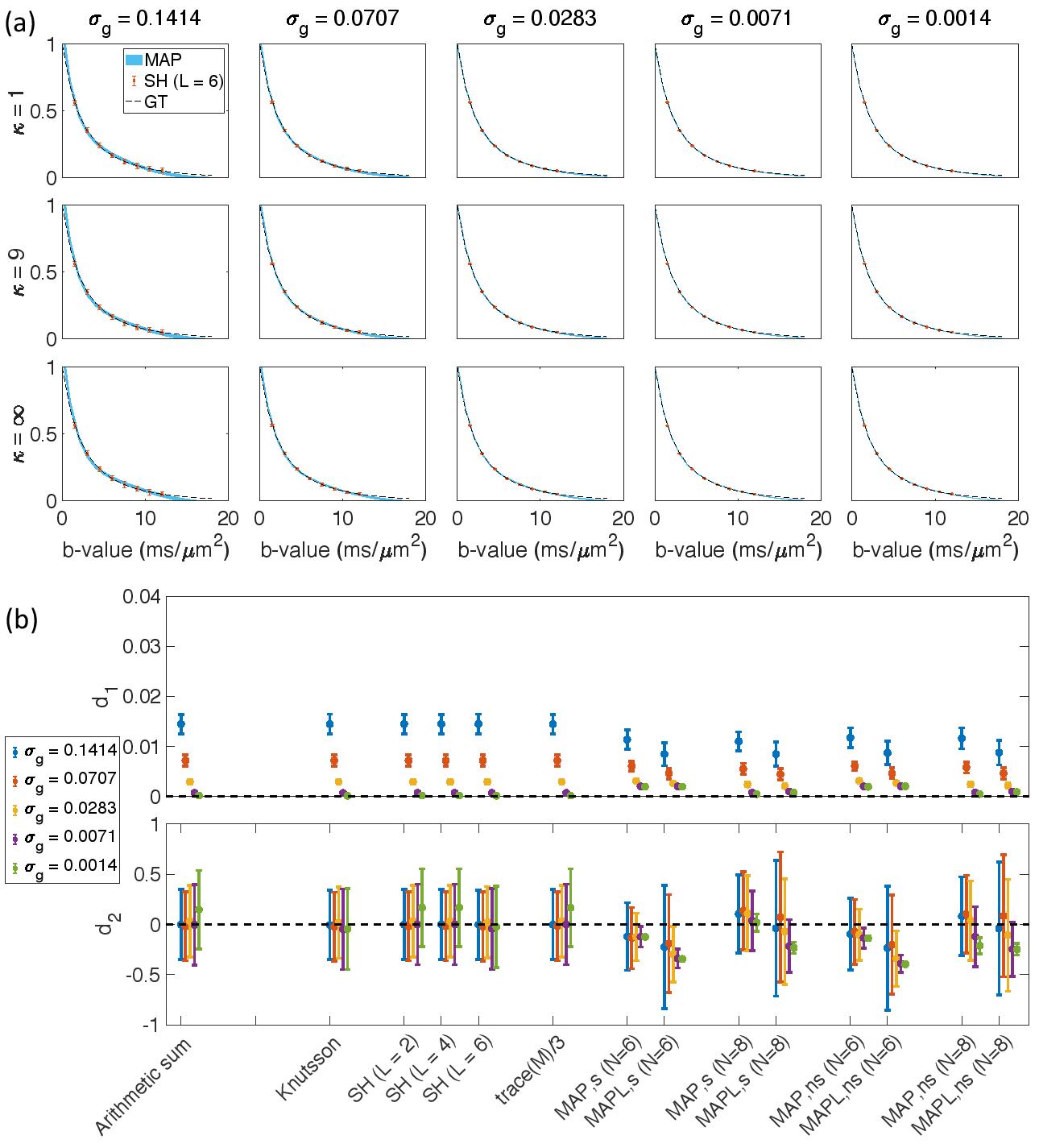
Fig. 1. The results from 488 samples for both shelled (61×8) and non-shelled point sets 18 in the presence of Gaussian noise. (a) the mean and std of the estimated signal versus b-value using MAP-MRI method with Nmax = 6 for five different noise floors, σg, and three different dispersion values, κ. The thickness of the blue band is twice the standard deviation of the signal estimates and its center is the mean. The dashed black line shows the ground truth and the red dots and bars show the results of the SH (L = 6). (b) the mean and std of the d1 and d2 measures for different methods.