Introduction

Hyperpolarized ¹³C magnetic resonance imaging (MRI) is a non-invasive imaging tool for assessing metabolism, including tumor lactate production^1,2 as well as metabolism profiles in the brain^3,4 and heart^5,6. Considering the finite decay and non-renewable magnetization generated by hyperpolarization, the single-shot spiral-out readout combined with spectral-spatial RF excitations is a common efficient technique to encode the k-space data⁷. However, the spiral readout is sensitive to B0 inhomogeneity, which results in image blurring⁸. Off-resonance correction methods have been applied in prior hyperpolarized ¹³C studies using spiral readouts, including 1)a multi-frequency automatic field map estimation scheme^8,9; 2)a model-based reconstruction to estimate the image and field map alternatively¹⁰. In this work, we improved the current off-resonance correction methods to self-estimate the field map and compared the performance in HP ¹³C studies in the different anatomies.

Methods

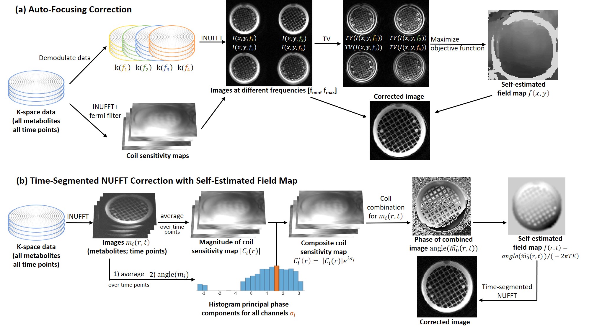
Auto-Focusing Correction
We modified the auto-focusing method with spiral readout for proton MRI⁸, and adapted this method to Hyperpolarized ¹³C data. The flowchart is shown in Figure 1(a). To begin with, the coil sensitivity maps were measured by smoothing the reconstructed pyruvate images. And the k-space data were demodulated at several frequencies with a suitable range to cover the estimated B0 inhomogeneity map. The field map can be estimated by maximizing the demodulated images ($$$I(x,y,f)$$$) with a total variation (TV) as the criteria, as shown below:$$
f(x,y)=\underset{f}{\mathrm{argmax}}\int\int_{A(x,y)}^{}{TV(I(x',y',f))dx'dy'}
$$Here, $$$A(x,y)$$$ is a summation window function at the location $$$(x,y)$$$. With the estimated field map, the corrected image was pieced together pixel by pixel from demodulated images ($$$I(x,y,f)$$$).
Time-Segmented NUFFT Correction with Self-Estimated Field Map
Considering the spiral readout, the image ($$$m_{i}(r,t)$$$) at $$$t$$$ time frame for $$$i$$$-th channel can be represented as $$
m_i(r,t)=m_0(r,t)C_i(r)e^{(-i2\pi f(r,t)TE)}
$$Where $$$C_i(r)$$$ is the coil sensitivity map of $$$i$$$-th channel, $$$f(r,t)$$$ is the off-resonance frequency. Estimation of field map is illustrated in Figure 1(b). Each channel image ($$$m_i(r,t)$$$) of all metabolites at all time points were reconstructed with NUFFT¹¹, then were averaged over time points. We estimated the phase produced by the coil by finding the phase ($$$\sigma_i$$$) with highest value from the histogram of averaged images. The magnitude ($$$\mid C_i(r) \mid$$$) of coil sensitivity map was extracted and then merged into the composite coil sensitivity map ($$$C_i^*(r)$$$) with the relationship$$
C_i^* (r)=|C_i (r)| e^{iσ_i}
$$The composite images ($$$\hat{m_0}(r,t)$$$) were then derived from the composite coil sensitivity map to estimate the field map by$$
f(r,t)=angle(\hat{m_0}(r,t))/(-2{\pi}TE)
$$Finally, corrected images were reconstructed with time-segmented NUFFT¹².
Phantom Experiments
Ethylene glycol (EG) phantom data were acquired on a 3T GE scanner using multi-slice 2D single-shot spiral readout to test the two self-estimated off-resonance correction methods. Data were acquired with a clamshell transmit coil and an 8-channel paddle receive array coil. Scan parameters were FOV=58X58cm², resolution=10.58X10.58mm², slice thickness=100mm, TE/TR=10/500ms, readout time=22ms, NEX=2400.
In-Vivo Experiments
We compared the two methods on different in-vivo anatomies: brain, heart, kidney. All in-vivo experiments were acquired on the 3T GE scanner with the same setting as the phantom experiment. In the in-vivo test, slice thickness=21mm, NEX=30. Other scan parameters were
1) brain experiments FOV = 39X39cm², resolution = 15X15mm², TE/TR = 10/125ms.
2) cardiac experiments FOV = 30X30cm², resolution = 12X12mm², TE/TR = 10/53ms.
3) renal experiments FOV = 75X75cm², resolution = 15X15mm², TE/TR = 10/100ms.

Results

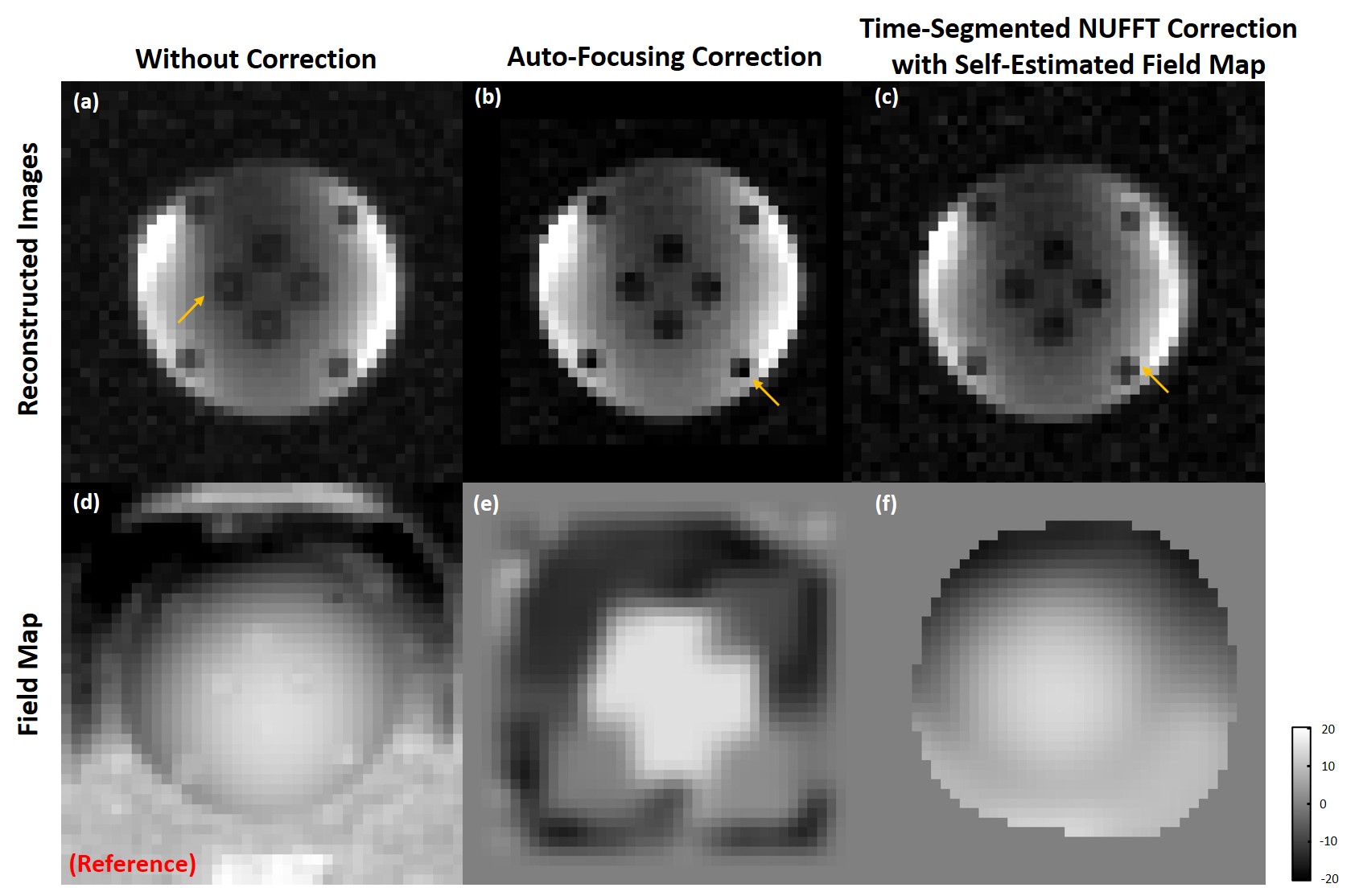
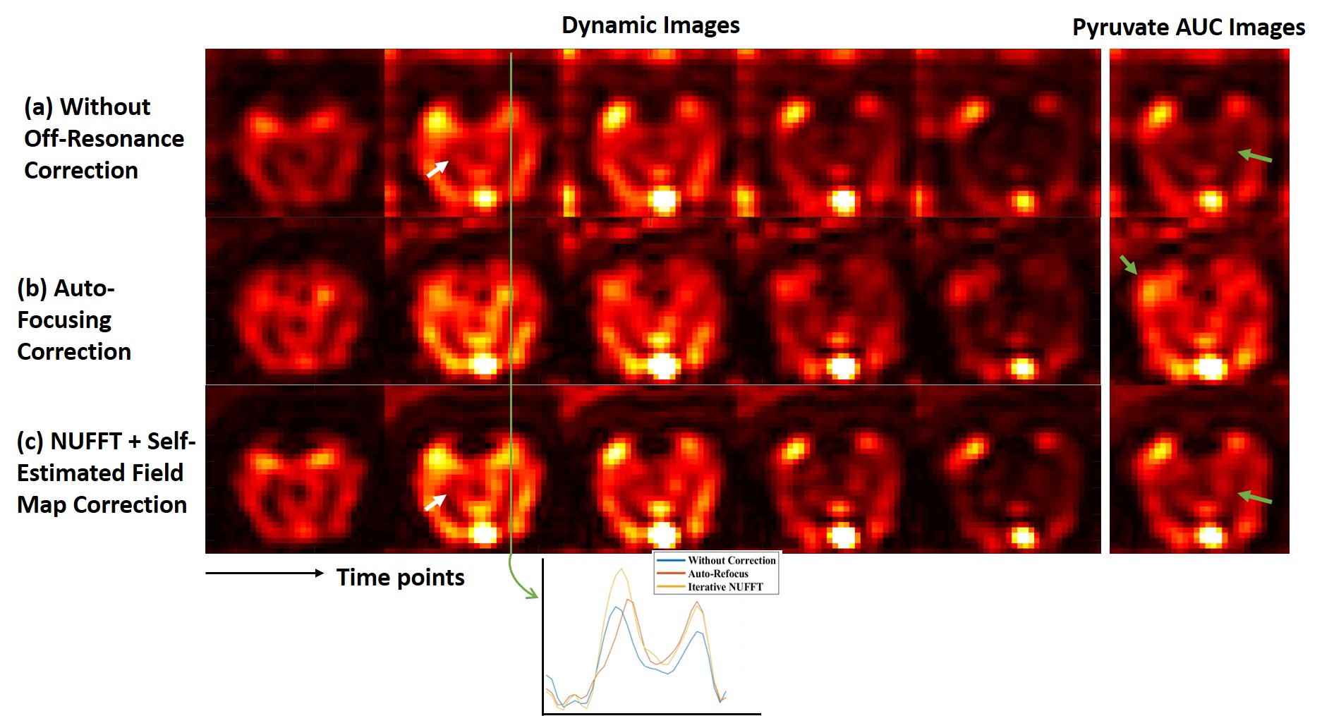
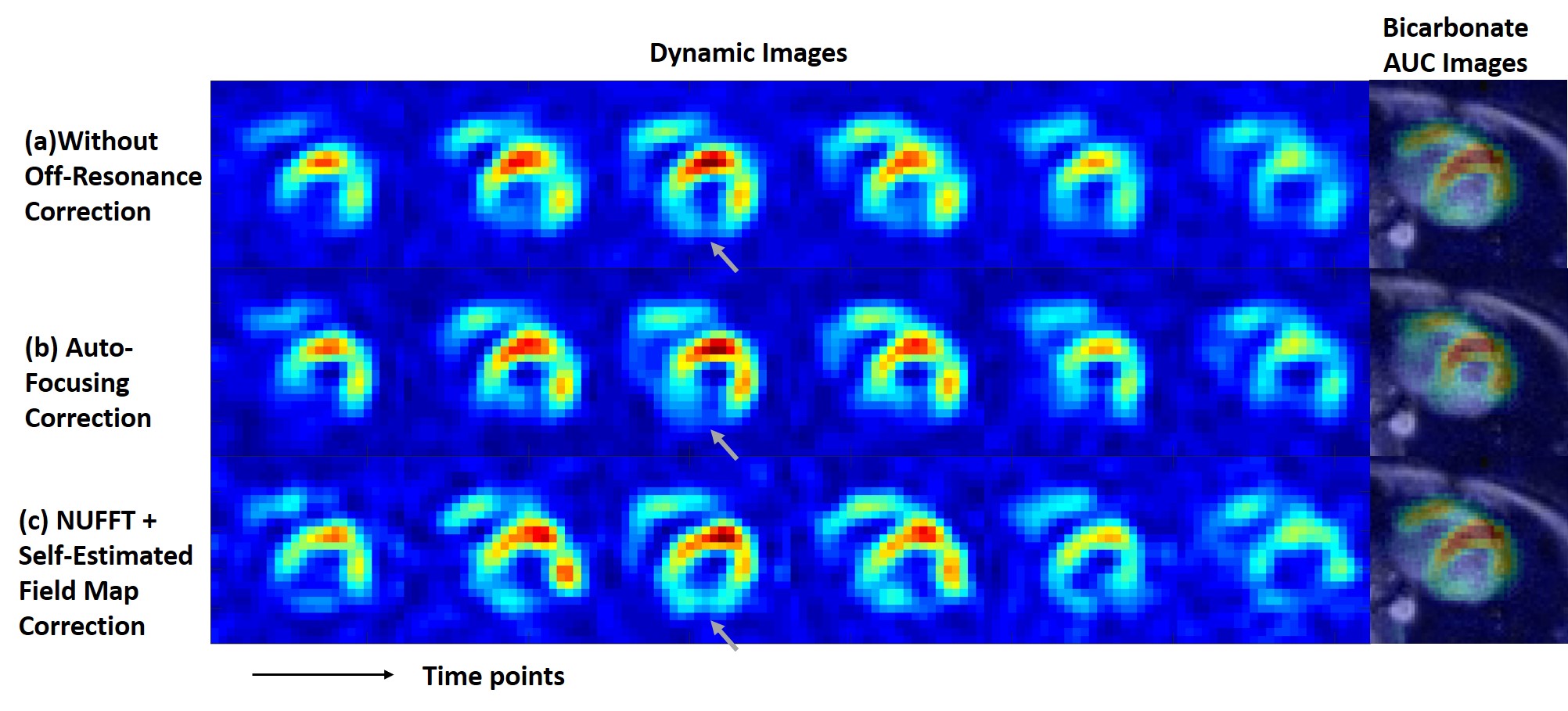
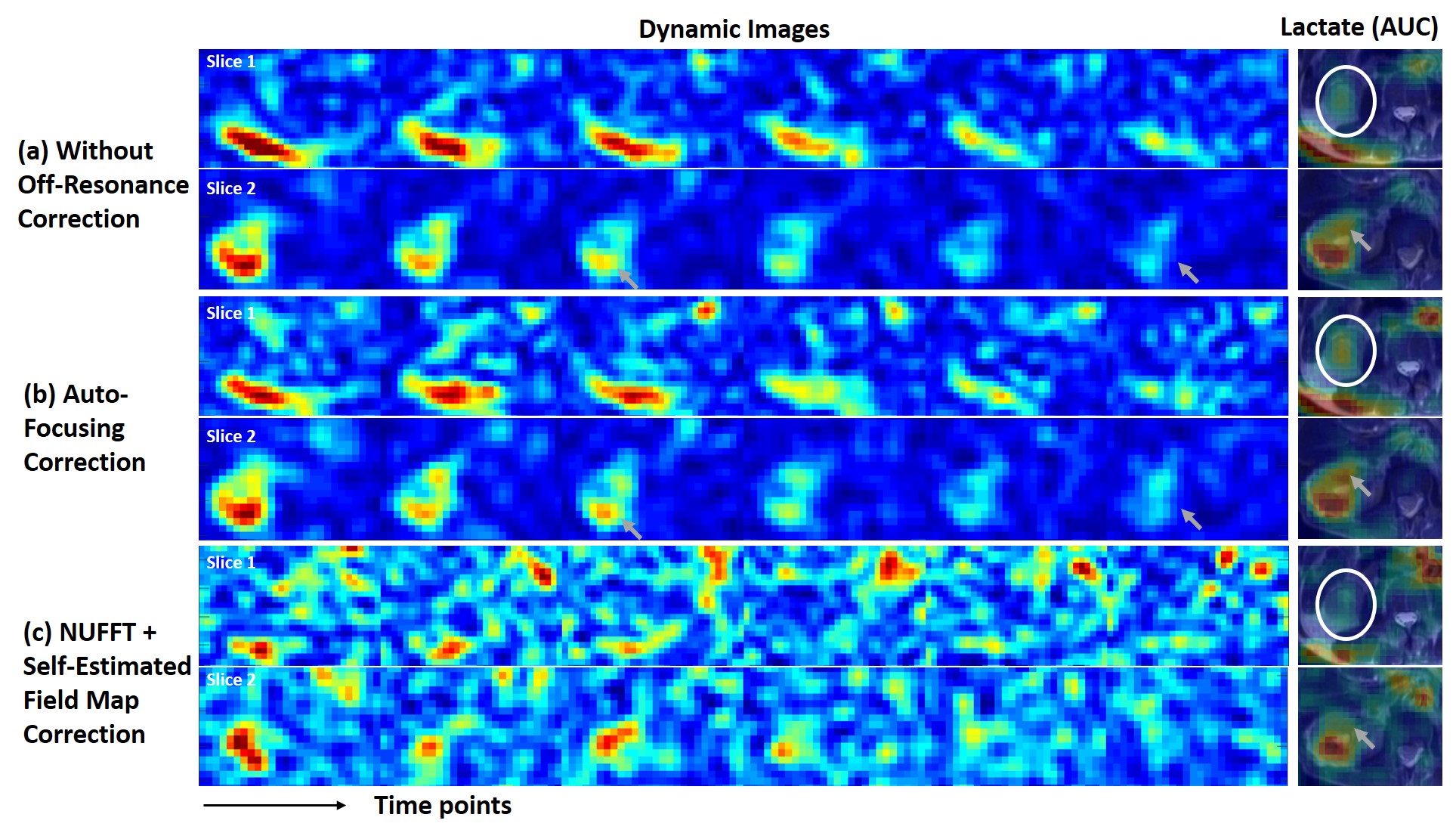
Figure 2 shows reconstructed images of EG phantom. Figure 3-5 show reconstruction results 13C pyruvate brain images, bicarbonate cardiac images and lactate renal images, respectively. Without off-resonance correction, the images have blurring at the edge between different materials, shown in Figure 2(a). In Figure 2, the auto-focusing correction method shows a better apparent correction performance with a sharper edge, indicated by the yellow arrows. However, the autofocus estimated field map is very different from the acquired field map while the time-segmented appears more accurate. In Figure 5, the auto-focusing correction method also shows a better correction performance with an intensity increase than the image without off-resonance correction, indicated by the white circles and grey arrows. In Figure 3&4, the self-estimated field map and time-segmented NUFFT correction method shows a better correction performance. In Figure 3, we chose a line profile to compare the intensity of three methods. The results of using the iterative NUFFT correction method has an improvement of intensity. In Figure 4, only using the method(c) provides visualize of the entire left ventricle myocardium, shown by the grey arrows.

Discussion

After comparing the results of two correction methods applying to different anatomies, the two methods are suitable for different regions. Considering the time-segmented NUFFT method may amplify the noise during iterations, this method is suitable for high SNR images. At the same time, the self-estimated field map is based on the assumption that the coil applies a constant phase on the image, so the estimated field map may have an offset frequency. The auto-focusing method uses a TV criteria to find the sharpest image, so this method is more suitable to clear structure images. And because the corrected image is pieced together, the SNR of corrected image should be same as the image reconstructed by the conjugate phase. In conclusion, the off-resonance effect in Hyperpolarized ¹³C data with spiral readout can be reduced by the self-estimated B0 inhomogeneity.

Acknowledgements

This work is supported by the National Institute of Biomedical Imaging and Bioengineering (P41EB013598, U01EB026412), Myokardia Myoseeds award, UCSF Resource Allocation Program, and American Cancer Society Research Scholar Grant 131715-RSG-18-005-01-CCE.