3556
Optimisation of MRI Bias Field Correction Algorithms on Whole Brain and Atrophy Measurements1Sydney Neuroimaging Analysis Centre, Sydney, Australia, 2University of Sydney, Sydney, Australia
Synopsis
Correction of bias fields is a common component in MRI analysis pipelines. We present a novel optimisation method to improve the white matter segmentation used for white matter weighted N4 correction, and validate using atrophy in a healthy control cohort.
Introduction
A crucial step in many structural MRI analysis pipelines is correction of low frequency intensity inhomogeneity, also known as bias fields. For many years, the gold standard approach to correct this bias field has been the N3 algorithm1, developed and made publicly available by the McConnell Brain Imaging Centre, Montreal Neurological Institute. The N3 algorithm employs a B-spline smoothing strategy to iteratively maximize the high frequency content of the distribution of tissue intensity, in essence filtering out the low frequency intensity variations associated with bias fields. This approach was built on and improved by Tustison et al. with their algorithm, N42. The changes implemented by Tustison et al. improved the performance of the algorithm at high field strength, where more significant bias fields are present, as well as allowing the input of a probabilistic mask to weight the voxels of distinct tissue during B-spline fitting, where initial tissue segmentation is required. However, the initial tissue segmentation can be biased from non-inhomogeneity corrected raw images. Given the importance of bias field correction in MRI tissue segmentation algorithms, and the use of tissue segmentation in N4 bias field correction, an iterative loop strategy can be developed to produce high quality WM probability map for optimal inhomogeneity correction outcome. In this study, we evaluated its performance on longitudinal whole brain and thalamic volumetric analysis, which commonly being used as imaging biomarker in neurodegenerative diseases.Methods
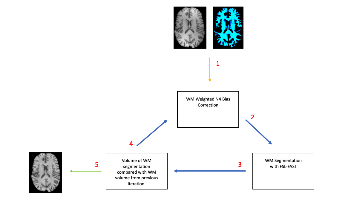
MR imaging data from 16 healthy controls was included in the analysis. Each subject completed 2 MRI session, separated by approximately 6 months. The imaging protocol included a volumetric 3D T1 weighted image (T1-WI) in both sessions. Bias correction was performed on the T1-WI using 4 methods (Figure 1): N3, N4, N4 with WM weighting (N4W) and N4 with iterative WM weighting (N4ITER). The N4ITER method is described further below and summarised in Figure 2. For each subject, percentage brain volume change (PBVC) between the two time-points was estimated using FSL-SIENA3. In this study, 0% brain volume change was assumed for all health control subjects over the 6-month time period. As the true PBVC direction (negative or positive) is not known, the main interest of this investigation was the absolute deviation from 0% volume change for each method. All percentage volume changes were thus converted to an absolute value prior to further analysis. All statistics were calculated with SPSS (Version 26.0. Chicago, SPSS Inc.). Any subjects with an annualised PBVC greater than 1.0% (as given by the mean PBVC from the 4 bias correction methods) were excluded from the subsequence statistical analysis, resulting in the exclusion of 3 subjects.Iterative WM N4 Bias Correction:
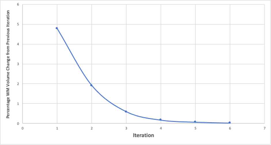
As summarised in Figure 2, an initial WM mask was generated by running FSL-FAST4 on the native T1-WI, without bias correction, and used for WM weighted N4 correction. The N4 corrected image was then segmented again with FSL-FAST, and the resultant WM masks fed back into the N4 algorithm to apply N4 correction, now weighted with the updated WM mask. For each iteration, N4 correction was applied to the original T1-WI, the only change to the input was the updated WM mask. After each tissue segmentation, the volume of WM was calculated from the WM PVE mask and compared to the previous iteration. If the change in WM volume was less than 0.05%, the process was terminated and a final WM weighted N4 correction was performed using the final WM mask (Figure 3).
Results
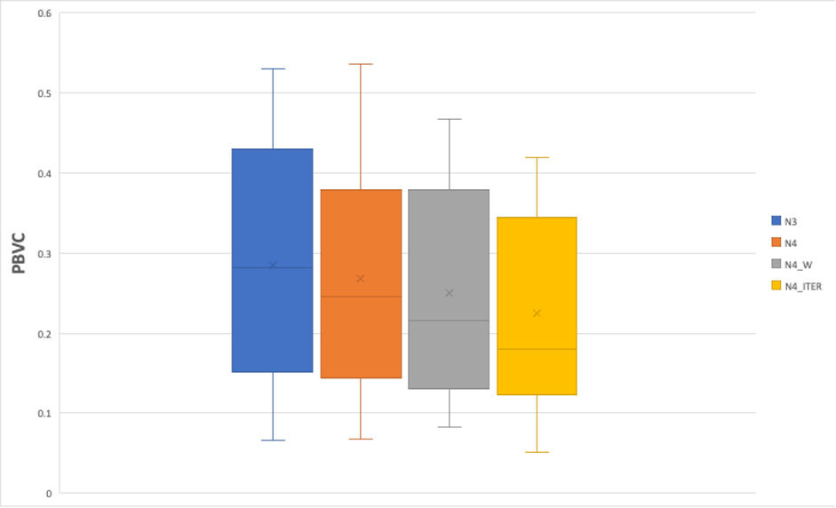
The mean PBVC for each bias correction method are displayed in Figure 4. The images corrected with the N4ITER resulted in the lowest mean PBVC (0.22%), and N3 corrected resulted in the greatest mean PBVC (0.28%). While the mean PBVC of images corrected with N4W also showed a reduced volume change (0.25%) compared with N3, the PBVC was greater than N4ITER and a paired t-test showed that the difference in mean PBVC between N4W and N4ITER was statistically significant (p = 0.009).Discussion
Estimation of whole brain and brain substructure volume changes are a common component in the analysis of many neurological disorders, and there is an increasing desire to include such quantitative and easily interpretable measurements in routine clinical practice. In the realm of moderate atrophy (<1% annually), estimated volume changes are dominated by technical variation5. Thus, the iterative N4 bias correction method introduced here provides a means to reduce the variance in PBVC changes introduced by bias fields, potentially allowing for more precise measurements of brain atrophy. Future studies with a larger sample size could provide more information on the impact of bias correction to brain substructure segmentation, however we demonstrate here the relevance of bias correction for registration-based tissue segmentation methods such as FSL-SIENA, which were influenced by bias field correction methods.Conclusion
We introduce here a novel iterative N4 technique for bias field correction, and validate the effectiveness with more accurate PBVC estimation in healthy controls. We also demonstrate the need for further investigation into the effects of bias correction methods on brain tissue segmentation.Acknowledgements
No acknowledgement found.References
1.Sled JG, Zijdenbos AP, Evans AC. A nonparametric method for automatic correction of intensity nonuniformity in mri data. IEEE Trans Med Imaging. 1998;17(1):87-97. doi:10.1109/42.668698
2. Tustison NJ, Cook PA, Gee JC. N4Itk. 2011;29(6):1310-1320. doi:10.1109/TMI.2010.2046908.N4ITK
3. Smith SM, Zhang Y, Jenkinson M, et al. Accurate, robust, and automated longitudinal and cross-sectional brain change analysis. Neuroimage. 2002;17(1):479-489. doi:10.1006/nimg.2002.1040
4. Zhang Y, Brady M, Smith S. Segmentation of brain MR images through a hidden Markov random field model and the expectation-maximization algorithm. IEEE Trans Med Imaging. 2001;20(1):45-57. doi:10.1109/42.906424
5. Narayanan S, Nakamura K, Fonov VS, et al. Brain volume loss in individuals over time: Source of variance and limits of detectability. Neuroimage. 2020;214(March). doi:10.1016/j.neuroimage.2020.116737
Figures