3551

Off-resonance correction of non-cartesian SWI using internal field map estimation

Guillaume Daval-Frérot^1,2,3, Aurélien Massire¹, Mathilde Ripart², Boris Mailhe⁴, Mariappan Nadar⁴, Alexandre Vignaud², and Philippe Ciuciu^2,3
¹Siemens Healthcare SAS, Saint-Denis, France, ²CEA, NeuroSpin, CNRS, Université Paris-Saclay, Gif-sur-Yvette, France, ³Inria, Parietal, Palaiseau, France, ⁴Digital Technology and Innovation, Siemens Healthineers, Princeton, NJ, United States

Synopsis

Patient-induced inhomogeneities in the magnetic field cause distortions and blurring during acquisitions with long echo times, as in susceptibility-weighted imaging. Most correction methods require collecting an additional $$$\Delta{B_0}$$$ field map. To avoid that, we propose a method to approximate this field map using the single echo acquisition only. The main component of the observed phase is linearly related to $$$\Delta{B_0}$$$ and TE, and the relative impact of non-$$$\Delta{B_0}$$$ terms becomes insignificant with TE>20ms at 3T. The estimated 3D field maps, produced at 0.6 mm isotropic under 3 minutes, provide corrections equivalent to acquired ones.

Introduction

Susceptibility-weighted imaging (SWI)¹ is commonly used in high resolution brain venography or traumatic brain injuries for its sensitivity to venous blood. Long echo times (20-40 ms) are used to highlight susceptibility information, but also result in off-resonance artifacts amplification causing geometric distortions and image blurring. Those effects are accumulated over the readout directions, notably affecting non-Cartesian sampling patterns which have recently gained popularity through compressed-sensing reconstruction^2,3 by allowing better spatial resolution and faster acquisitions. Therefore off-resonance correction appears essential to bring these methods to clinical practice.

Most non-specific correction methods, such as [4], require the prior knowledge of the $$$\Delta{B_0}$$$ map, resulting in an additional low-resolution MR acquisition and a counterproductive increase in total examination time. While at least two echo times are usually needed to produce a field map, we propose to only use the phase images of the SWI acquisition, benefiting from high spatial resolution, robustness to inter-scan motion and with minimal impact on reconstruction time. Our method follows a recent study in EPI⁵ where an initial field map is updated over time using solely the acquired phase. Similarly, the main challenge was to unwrap the phase of the volume and required exploring several algorithms^6-8 .

Materials and methods

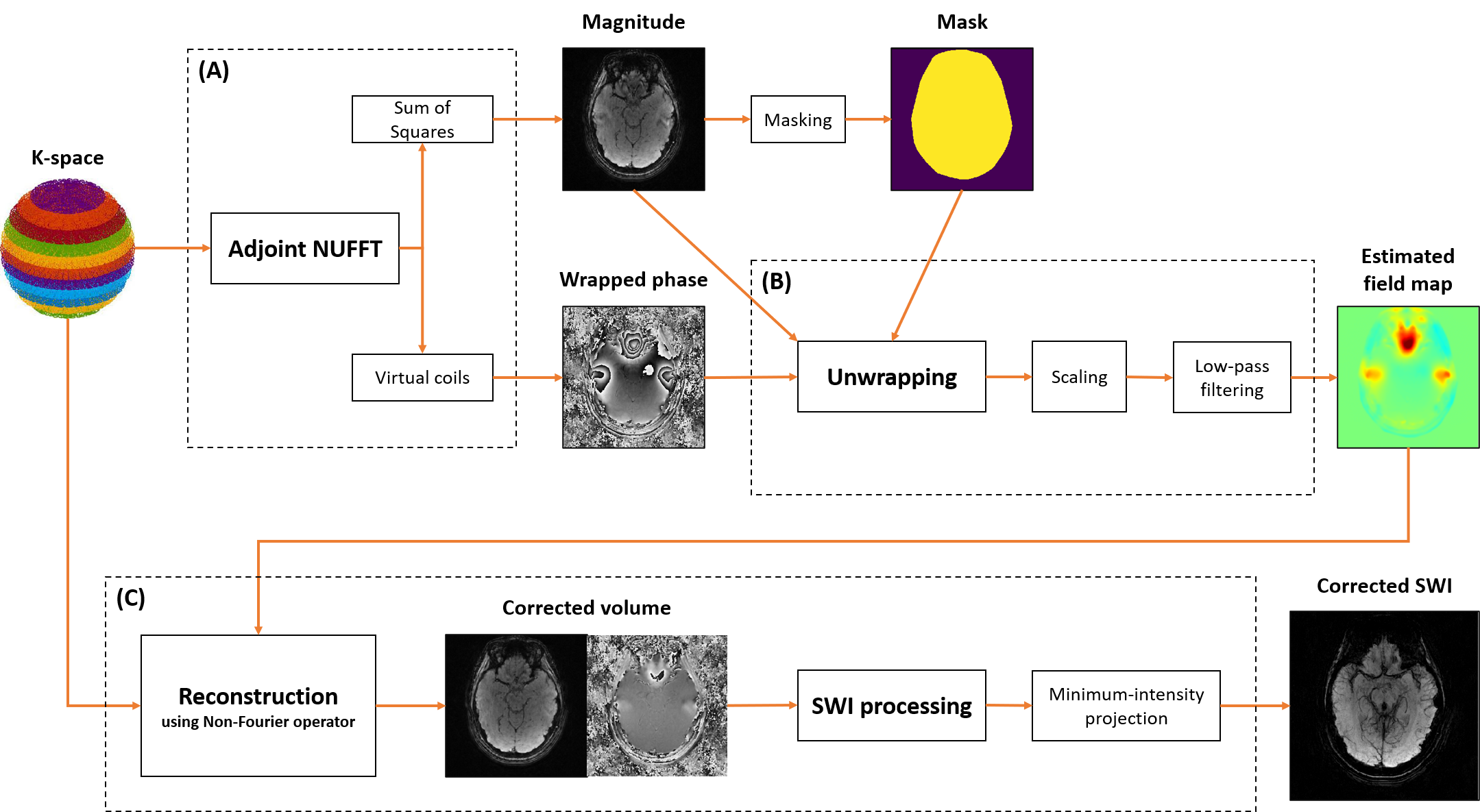
The phase of the MR image can be formulated voxelwise as follow: $$$\varphi = \varphi_0 + 2\pi{TE}\Delta{B_0}$$$. Our approach consists in approximating the field map as $$$\Delta{B_0} = \varphi / 2\pi{TE}$$$, considering other contributions are negligible for long TE at intermediate field. The $$$\varphi_0$$$ term gathers the effects of different sources such as heating, motion, radio frequency pulse heterogeneities, coil sensitivities and eddy current. Based on literature, heating⁹ and physiological motion¹⁰ contributions can be neglected. As bulk motion would also impact the acquisition, it is assumed to be addressed separately. Contributions from the RF fields (emission and reception) are limited¹¹ and correctable¹², respectively. Eddy currents are also weak for well-designed and calibrated MR scanners¹¹. Overall, these contributions to $$$\varphi_0$$$ were estimated about 15-20 times^11,13 lower than $$$2\pi TE \Delta{B_0}$$$ at 3T with TE=20ms.

The calculated $$$\Delta{B_0}$$$ maps were processed as shown in Fig. 1A-1B. The magnitude and wrapped phase are obtained by computing the adjoint of the density compensated k-space data. The key step was to unwrap the phase (see Fig. 2A). The algorithm introduced in [6] was preferred over the Laplacian method⁸ for its consistency. It similarly solves a Poisson equation weighted by the magnitude of the image previously estimated. Finally, the phase was rescaled and a Hanning filter was applied to filter out high frequencies to avoid suppressing the susceptibility contributions.

A SWI volume was acquired for each of the two volunteers at 3T with a 64-channel head/neck coil array using the recently proposed 3D Spherical Stack-of-SPARKLING² sampling pattern. Acquisition parameters were the following: TA: 5min, 0.6mm isotropic resolution, FOV: 240mm, slice number: 208, TE/TR: 20/37ms, Bw: 33Hz/px. An additional reference $$$\Delta{B_0}$$$ map was acquired with the following parameters: TA: 2min43s, same FOV, 2mm isotropic resolution, TE1/2: 4.92/7.38ms.

Image reconstructions (see Fig. 1C) were performed iteratively³ in 3D, with a soft thresholding regularization in the wavelet domain. The correcting non-Fourier operator introduced in [4] was used with a pre-computed density compensation. The channels were re-combined as in Fig. 1A using sum-of-squares (magnitude) and virtual coils¹² (phase). Reconstructions were performed without correction, and with correction using either acquired or estimated field maps. SWI minimum-intensity projection was applied over 16mm. All post-processing was run on a 2560 cores Quadro P5000 GPU and 16GB of GDDR5 VRAM.

Results

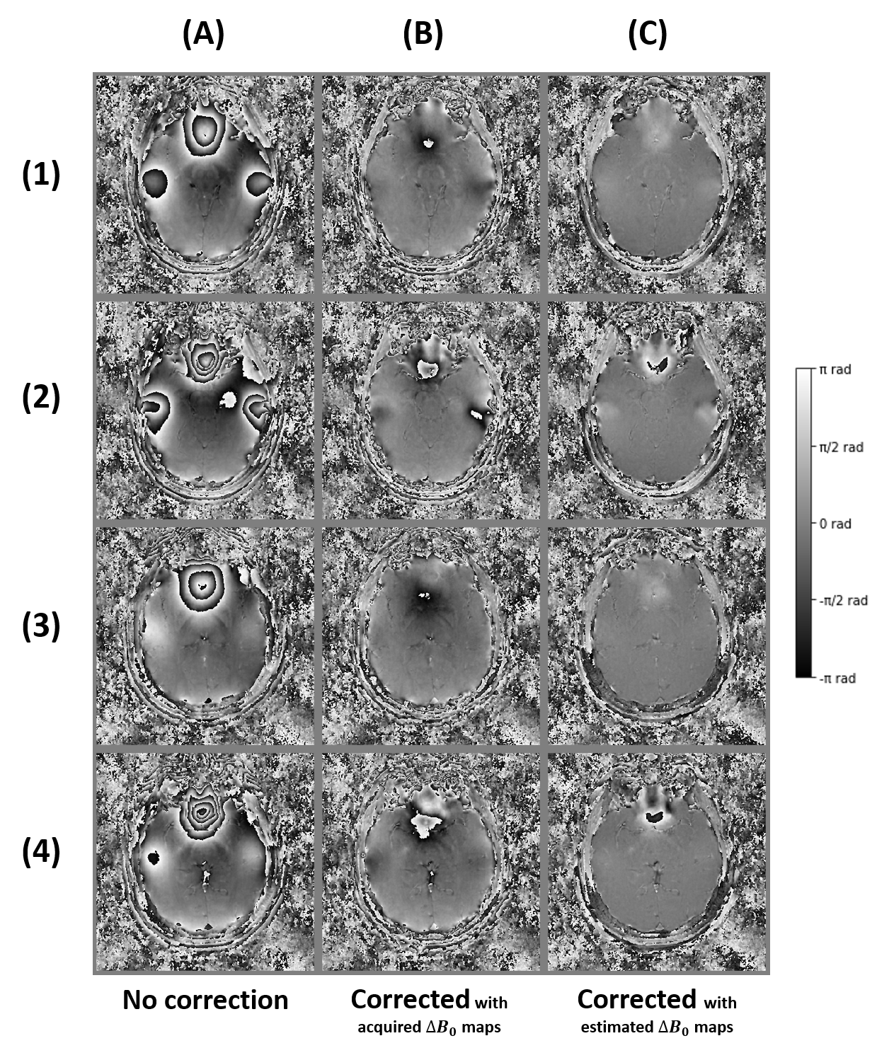
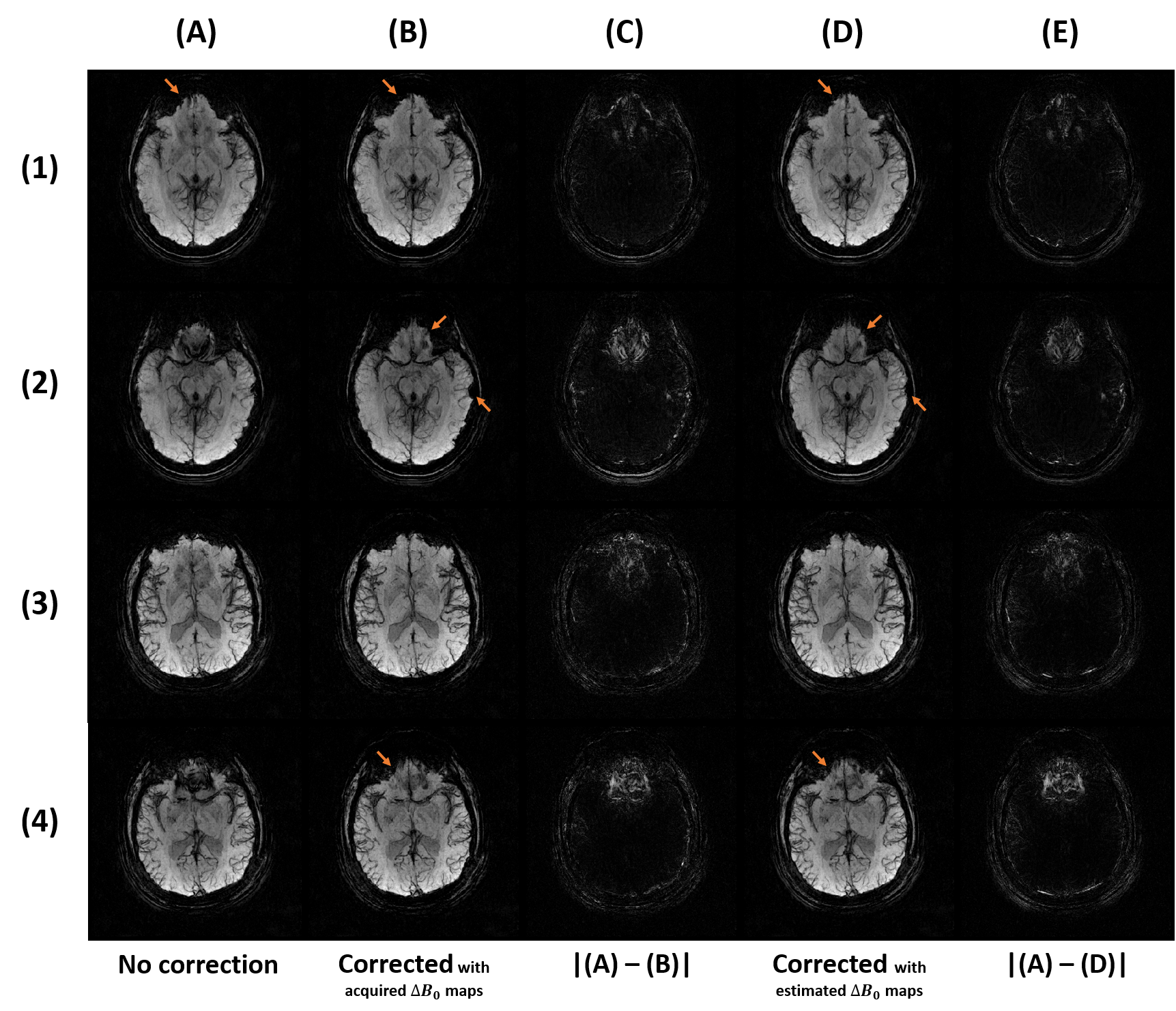
The field map estimation took under 3min: adjoint computation (127s), coil combination (31s), masking (5s), and phase unwrapping, filtering and scaling (12s). As shown in Fig. 2C, the chosen unwrapping algorithm is more consistent within the inner regions, with a slightly inferior range compared to acquired field maps. However, the phase maps displayed in Fig. 3B suggest that the values of the acquired field maps are too high as the phase is wrapped negatively, showing an overcompensation of the inhomogeneities. The estimated $$$\Delta{B_0}$$$ maps used for Fig. 3C produce better compensations but on the contrary slightly underestimated, likely because of the low-pass filtering. The resulting SW images in Fig. 4 show a similar correction between the reference (Fig. 4C) and the proposed pipeline (Fig. 4E), with modest differences in favor of the latter.

Conclusion

In the case of long echo times at intermediate field for a well-tuned MRI system, a single phase image can be used to quickly estimate a $$$\Delta{B_0}$$$ map, enabling corrections of off-resonance artifacts similar to those obtained using an additional $$$\Delta{B_0}$$$ acquisition. Both already have close durations, but the proposed method can be run offline with robustness to inter-scan motion and in high resolution. This duration could be further reduced even below the current acquisition time by including the low-pass filter during the adjoint call.

Acknowledgements

The concepts and information presented in this abstract are based on research results that are not commercially available. Future availability cannot be guaranteed. We thank Caroline Le Ster and Alexis Amadon for useful discussions, and Chaithya G R for prior contributions to the code.

References

[1] Haacke EM, Xu Y, Cheng YC, Reichenbach JR. Susceptibility Weighted Imaging (SWI). Magnetic Resonance in Medicine 2004; 52 (3): 612–18.

[2] Lazarus, C, Weiss P, El Gueddari L, Mauconduit F, Massire A, Ripart M, Vignaud A, Ciuciu P. 3D Variable-Density SPARKLING Trajectories for High-Resolution T2*-Weighted Magnetic Resonance Imaging. NMR in Biomedicine 2020; 33 (9): e4349.

[3] El Gueddari L, Ciuciu P, Chouzenoux E, Vignaud A, Pesquet JC. Calibrationless oscar-based image reconstruction in compressed sensing parallel MRI. 2019 IEEE 16th International Symposium on Biomedical Imaging (ISBI 2019) pp. 1532-1536.

[4] Sutton, BP, Noll DC, and Fessler JA. Fast, Iterative Image Reconstruction for MRI in the Presence of Field Inhomogeneities. IEEE Transactions on Medical Imaging 2003;22 (2): 178–88.

[5] Dymerska B, Poser BA, Barth M, Trattnig S, Robinson SD. A Method for the Dynamic Correction of B0-Related Distortions in Single-Echo EPI at 7T. NeuroImage, Neuroimaging with Ultra-high Field MRI: Present and Future, 2018; 168: 321–31.

[6] Ghiglia DC, Romero LA. Robust Two-Dimensional Weighted and Unweighted Phase Unwrapping That Uses Fast Transforms and Iterative Methods. JOSA A 1994; 11: 107–17.

[7] Herráez MA, Burton DR, Lalor MJ, Gdeisat MA. Fast Two-Dimensional Phase-Unwrapping Algorithm Based on Sorting by Reliability Following a Noncontinuous Path. Applied Optics 2002; 41 (35): 7437.

[8] Schofield MA, Zhu Y. Fast Phase Unwrapping Algorithm for Interferometric Applications. Optics Letters 2003; 28 (14): 1194.

[9] Le Ster C, Mauconduit F, Mirkes C, Bottlaender M, Boumezbeur F, Djemai B, Vignaud A, Boulant N. RF Heating Measurement Using MR Thermometry and Field Monitoring: Methodological Considerations and First in Vivo Results. Magnetic Resonance in Medicine 2020.

[10] Van de Moortele PF, Pfeuffer J, Glover GH, Ugurbil K, Hu X. Respiration-Induced B0 Fluctuations and Their Spatial Distribution in the Human Brain at 7 Tesla. Magnetic Resonance in Medicine 2002; 47 (5): 888–95.

[11] Lier A, Brunner DO, Pruessmann KP, Klomp D, Luijten PR, Lagendijk J, Berg C. B1+ Phase Mapping at 7 T and Its Application for in Vivo Electrical Conductivity Mapping. Magnetic Resonance in Medicine 2012; 67 (2): 552–61.

[12] Parker DL, Payne A, Todd N, Hadley JR. Phase Reconstruction from Multiple Coil Data Using a Virtual Reference Coil. Magnetic Resonance in Medicine 2014; 72 (2): 563–69.

[13] Setsompop K. Design Algorithms for Parallel Transmission in Magnetic Resonance Imaging. 2009.

Figures

Figure 1 : Pipeline of the field map estimation followed by an off-resonance correction. The magnitude and associated mask estimated with the adjoint are used to weight and stabilize the phase unwrapping algorithm.

Figure 2 : Comparison of field maps estimated using different unwrapping algorithms. Slices (1) and (2) from two different volumes were chosen to show the limitations of the different algorithms. (A) is the phase before unwrapping. (B) is the acquired field map. (C), (D) and (E) are respectively obtained with the methods described in [6], [7] and [8].

Figure 3 : Comparison of the reconstructed phases without correction (A), with correction using the acquired field map (B) and with correction using the estimated field map (C) arranged by slices. The wrapped regions in (A) give a raw idea of the inhomogeneities, since without other effects than $$$\Delta{B_0}$$$ the phase should ideally be null except for the susceptibility of iron.

Figure 4 : Comparison of the SWI with mIP without correction (A), with correction using the acquired field map (B) and with correction using the estimated field map (D) with the same slices as Fig3. (C) and (E) are respectively the difference between (A) and (B), and between (A) and (D).

Proc. Intl. Soc. Mag. Reson. Med. 29 (2021)

3551