Introduction

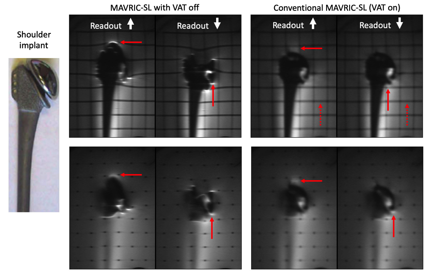
Orthopedic metallic implants are used extensively to treat late stage osteoarthritis, degenerative disc disease, and stabilize fractures following trauma. Multispectral imaging (MSI) sequences (e.g. SEMAC¹, MAVRIC-SL²) are used to investigate complications near metallic implants and inform surgical planning. MSI sequences employ the view-angle tilting (VAT) sequence modification³ to eliminate geometric distortion caused by severe B0 inhomogeneity in the vicinity of metal (Figure 1). However, VAT results in readout blurring^4,5 and residual intensity-based artifacts persist⁶. The purpose of this work is to address these limitations of MSI for the purposes of artifact correction near metallic implants. This is done by jointly estimating the image content and field inhomogeneity from spectral subimages acquired with a dual polarity readout scheme.

Methods

The signal $$$s$$$ at position $$$\overrightarrow{r}=(x,y,z)$$$ in each spectral subimage $$$b$$$ is modelled as a non-linear function of the image content $$$m$$$ and field inhomogeneity $$$f$$$ along the readout dimension $$$x$$$ as follows.

$$s(\overrightarrow{r},b)=\int m(\overrightarrow{r})\cdot RF(f(\overrightarrow{r})+\gamma G_z z-f_b)\cdot PSF(x-x'-\frac{f(\overrightarrow{r})-f_b}{\gamma G_x})dx'$$

In this equation $$$RF(f)$$$ is the $$$B_1$$$ envelope, $$$f_b$$$ is the center frequency of bin $$$b$$$, $$$PSF(x)$$$ is the point spread function along the readout dimension and $$$G_x, G_z$$$ are the readout and slice-select gradients respectively. The $$$f_b$$$ term in the argument of the PSF encapsulates the effect of VAT on spatial encoding.

The above forward model is discretized by modelling the subject as being composed of $$$d$$$ uniformly spaced point sources per voxel ($$$d=4$$$ is used in this work). Sub-voxel image content and field are modelled as piece-wise constant and piece-wise linear across the voxel. Equation 2 describes this model with $$$i,j$$$ indexing the voxel and subvoxels, respectively.


$$s(x,z,b)=\sum_{i,j}m_{i,j}\cdot RF(f_{i,j}+\gamma G_z z-f_b)\cdot PSF(x-x_{i,j}-\frac{f_{i,j}-f_b}{\gamma G_x})$$

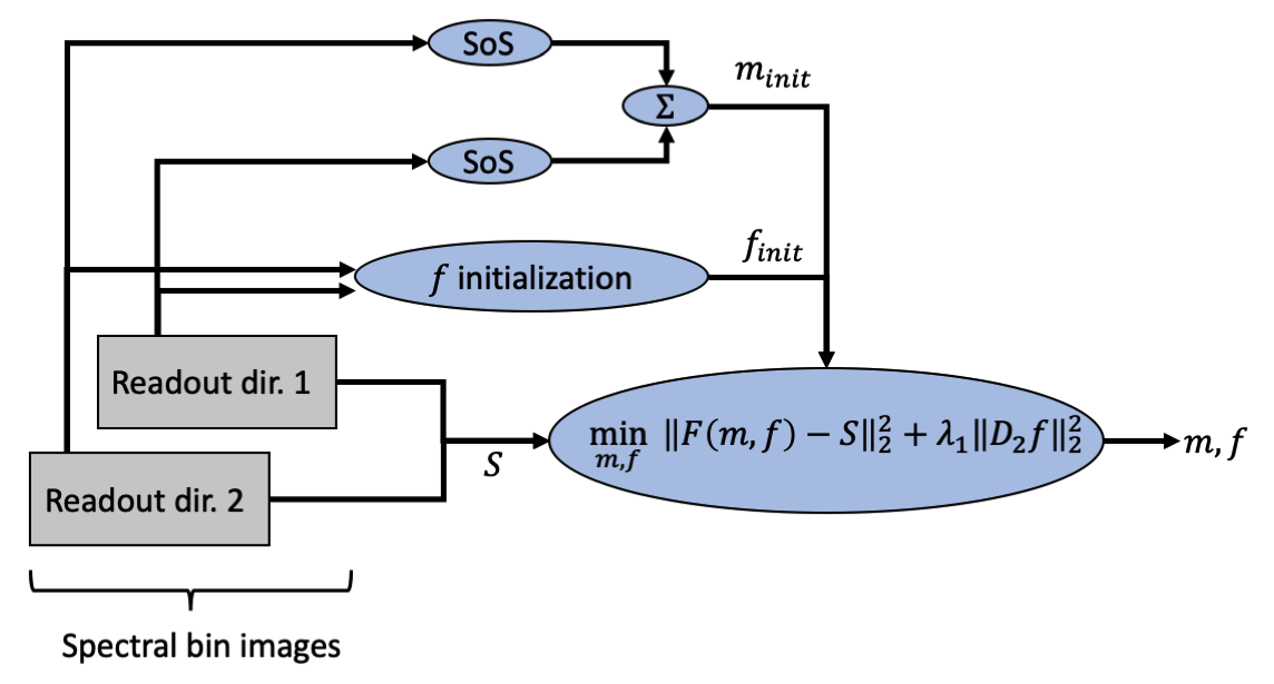
We formulate the estimation of parameters $$$m_i$$$ and $$$f_i$$$ as a regularized non-linear least squares (NLLS) problem with a forward model $$$F$$$ mapping $$$m,f$$$ to a set of measurements $$$S$$$ according to equation 2. The NLLS problem is regularized with the second derivative of $$$f$$$. The complete objective is given in Figure 2. The NLLS problem is solved with a Gauss-Newton approach implemented in Python using the scipy.optimize library. Regularization parameter $$$\lambda=1$$$ was used throughout all experiments after a limited grid search.

The proposed method is investigated in both digital and physical phantoms. All phantom data was acquired with a MAVRIC-SL sequence played twice to measure each spectral bin image with both positive and negative readout gradient polarity. Initialization of $$$m$$$ and $$$f$$$ is described in Figure 2. All images were acquired on a 3T GE Signa Premier. Acquisition parameters: voxel resolution 0.6x1.2x2.4 mm, matrix size 512x128x32, 2x PE acceleration, readout bandwidth per voxel 488.3 Hz, scan time 5:28 for one readout direction. In simulation, the matrix size is 128x50 with 500 Hz readout bandwidth per voxel.

Results

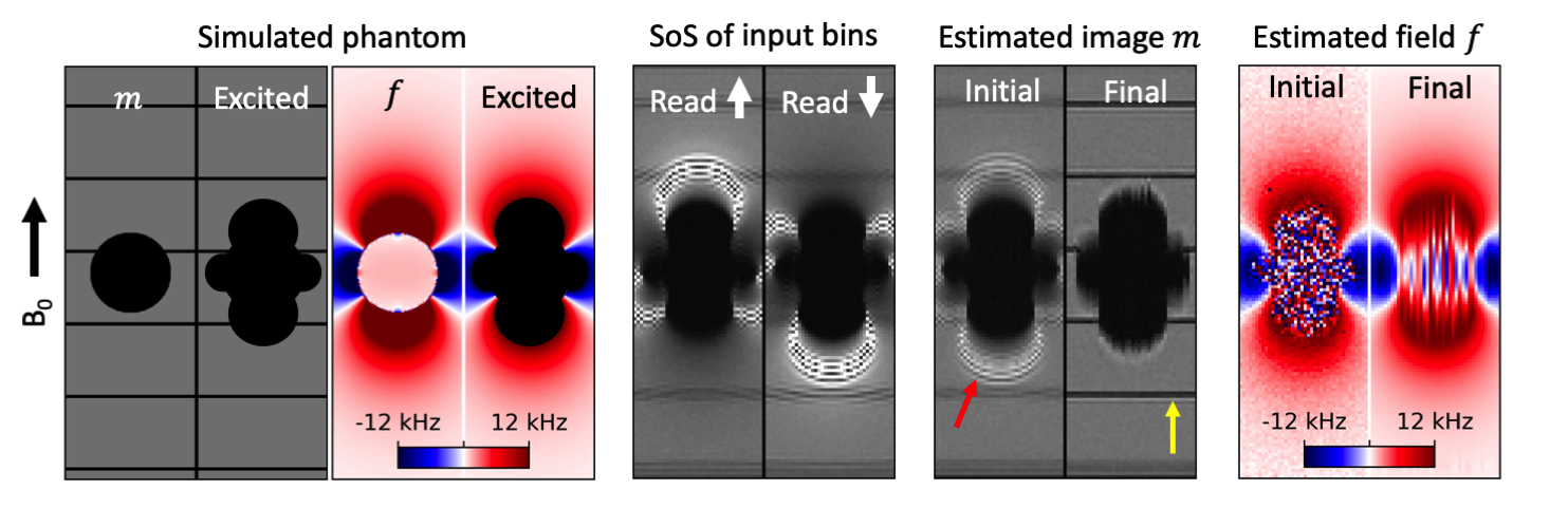
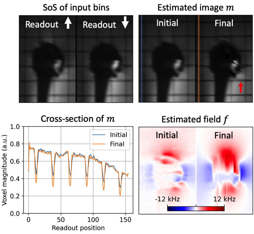
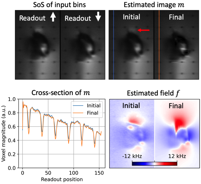
Results with the digital phantom are provided in Figure 3. Readout blur and intensity-based artifacts are clearly visible from the sum-of-squares (SoS) of spectral bins for both input datasets. Intensity artifacts in input data are eliminated in the final image, revealing grid lines that were previously obscured. A reduction in readout blur can also be observed by comparing the appearance of grid lines between panels. Image recovery at the edges of the excited region appears less smooth in the estimated image.

Figures 4 and 5 show results for two slices in the shoulder phantom. Readout blur is clearly reduced, resulting in sharper horizontal grid lines in the estimated image. In Figure 4, intensity artifacts are minor and the final estimation provides no appreciable improvement in this regard. The edges of the implant appear less smooth in the final estimation as compared to the initial state. In Figure 5, intensity artifacts are more significant and the final estimation result most notably removes a ripple artifact above the implant head.

Discussion

Conditioning of the inverse problem is a key consideration for this work. Dual polarity readout data is necessary to separate pile-up intensity artifacts, but in practice it was found not to be sufficient without regularization. Artifacts of the regularization manifest as over-smoothing of details in the field map.

The proposed method requires a doubling of the number of measurements (to acquire both readout directions) in order to achieve adequate conditioning for the inverse problem, however the SNR efficiency appears to be maintained (comparing perceived SNR in initial and final panels). Recent developments to accelerate MSI data acquisition^8,9 may be combined with this work to reduce overall scan time.

Conclusion

The proposed method mitigates readout blur caused by VAT and demonstrates the capacity to correct intensity artifacts in some places. Future work is needed to improve stability around the edges of the excited region.

Acknowledgements

Research support provided by R01 EB017739 and GE Healthcare.