3539
Realistic Simulation of MRI Metal Artifact and Field Strength Dependence1Electrical and Computer Engineering, University of Southern California, Los Angeles, CA, United States, 2Radiology, Stanford University, Stanford, CA, United States, 3Electrical Engineering, Stanford University, Stanford, CA, United States, 4Bioengineering, Stanford University, Stanford, CA, United States, 5Biomedical Engineering, University of Southern California, Los Angeles, CA, United States
Synopsis
MRI near metallic implants suffers from severe artifacts due to magnetic susceptibility, and these artifacts scale with the B0 field strength. Techniques like “view angle tilting” and “multi spectral imaging” partially mitigate these distortions and are widely used at 1.5T and 3T. Here, we provide a pipeline for realistic simulation of MRI metal artifacts and noise using anatomic digital phantoms and susceptibility calculations. For one example application, total hip arthroplasty, we demonstrate the impact of field strength (0.2T, 0.55T, 1.5T, 3T), and MSI parameters such as receiver bandwidth, RF bandwidth, and number of spectral bins.
INTRODUCTION
Orthopedic metallic implants are used extensively to treat late-state osteoarthritis, degenerative disc disease, and fracture stabilization following trauma or resection. In the United States, roughly 7 million patients were living with a hip or knee replacement in 2010, and this number is increasing each year1. There is an unmet need to better image tissues immediately adjacent to the metallic implants, for patient follow-up and to identify possible complications. MRI in these locations is limited by the susceptibility difference between metallic implants and human tissues, which causes substantial artifacts and distortions2. Since this difference produces B0 dependent field variations, field strength has a large impact on size of metal artifacts. Techniques like view angle tilting (VAT) and multi spectral imaging (MSI) can partially mitigate these effects and are now widely used at 1.5T and 3T. MSI sequence parameters such as receiver bandwidth, RF bandwidth, and number of spectral bins also impact the amount of residual artifact.Here, we demonstrate a framework capable of simulating the effects of field strength, and MSI parameters on metal artifacts, and apply it to the example case of imaging after total hip arthroplasty (THA). This is based on the digital XCAT body phantom3, a digital hip implant phantom, and realistic noise that is calibrated based on 3T measurements.
METHODS
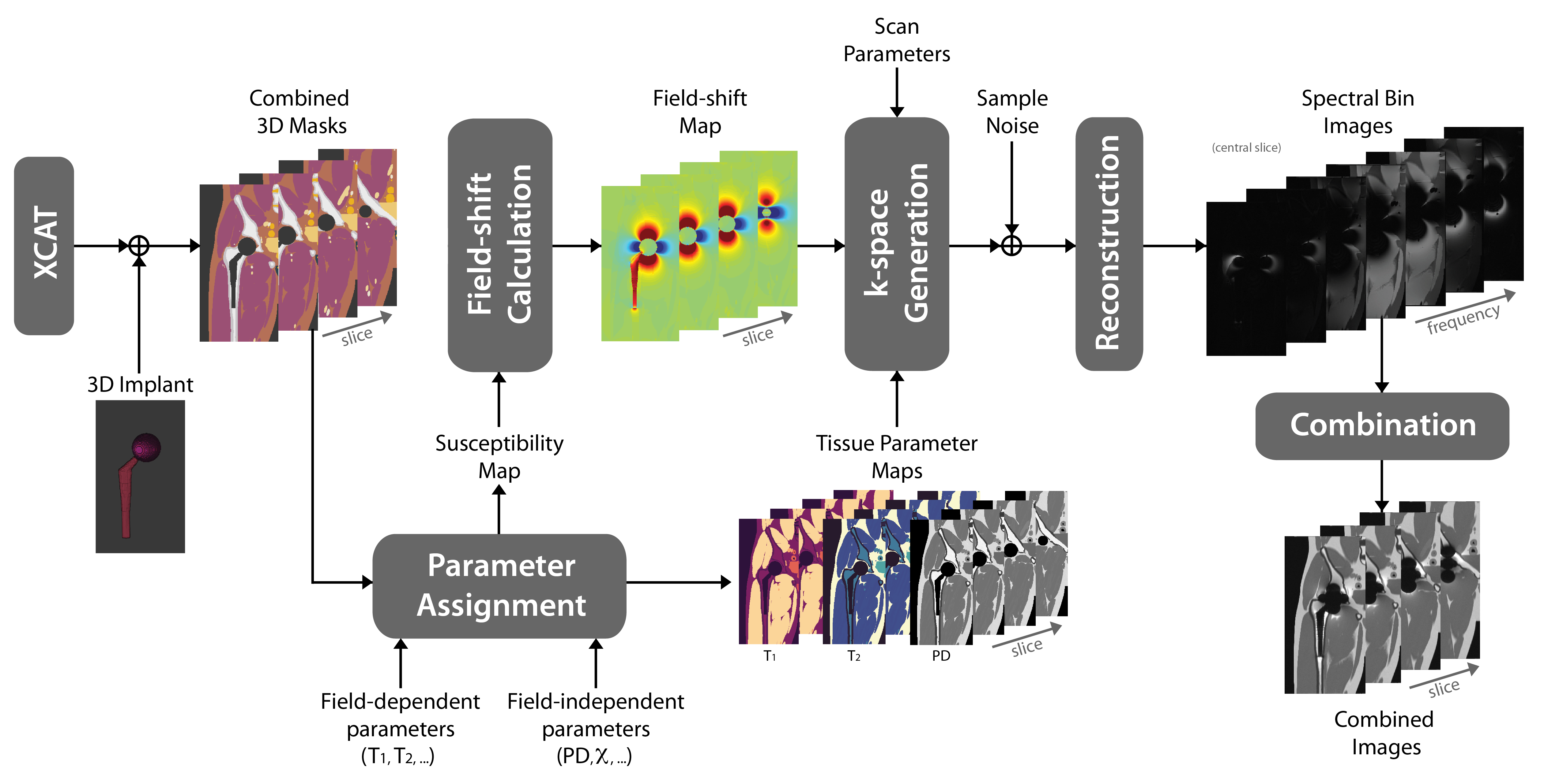
Realistic AnatomyWe start with the 3D XCAT 3434 adult male body phantom3, and digitally insert a 3D hip implant phantom with a cobalt-chromium head and a titanium stem4. Proton density (PD), and susceptibility values are assigned to tissue masks5. In this work, only PD-weighted imaging is considered. However, other contrasts can also be simulated when field dependent values of T1 and T2 are assigned to tissue masks6–9.
Metal MRI Simulation
Figure 1 illustrates the simulation pipeline. The susceptibility-induced field shift is calculated using a Fourier-based convolution method10. Imaging parameters: FOV 40x20x60cm3; resolution 1x1x3mm3; number of slices 20; Cartesian sampling; single body coil, homogeneous B1+ and B0. We simulate a PD-weighted MAVRIC-SL sequence11 with parameters: phase encoding in the left-right and anterior-posterior directions, spectral bins with Gaussian spectral profile, and 1kHz bin separation4. Bin images are combined with quadrature-summation.
Realistic Noise
Noise levels were calibrated using a reference dataset obtained with MAVRIC-SL at 3T, with parameters: RF bandwidth=2.25kHz, readout bandwidth/pixel=625Hz. Additive bivariate gaussian data was added to synthesized k-space data to match SNR of thigh muscle closest to the femur bone of the 3T dataset. Signal strength was scaled using $$$(B_0/B_{0,ref})^2$$$ and noise standard deviation is scaled with $$$(B_0/B_{0,ref})\sqrt{BW/BW_{ref}}$$$ where ref represents the reference acquisition12 ($$$B_{0,ref}$$$=3T and $$$BW_{ref}$$$=625Hz).
Experimental Methods and Data Analysis
Simulations were performed for: B0=0.2T,0.55T,1.5T,3T; RF bandwidth= 0.5kHz,1kHz,2kHz,2.25kHz; readout bandwidth/pixel= 250Hz,500Hz,625Hz,1kHz; total number of bins=12,18,24. We evaluate image quality of a central coronal slice by several metrics: artifact left-right extent (mm), artifact area (mm2), and SNR (dB).
RESULTS
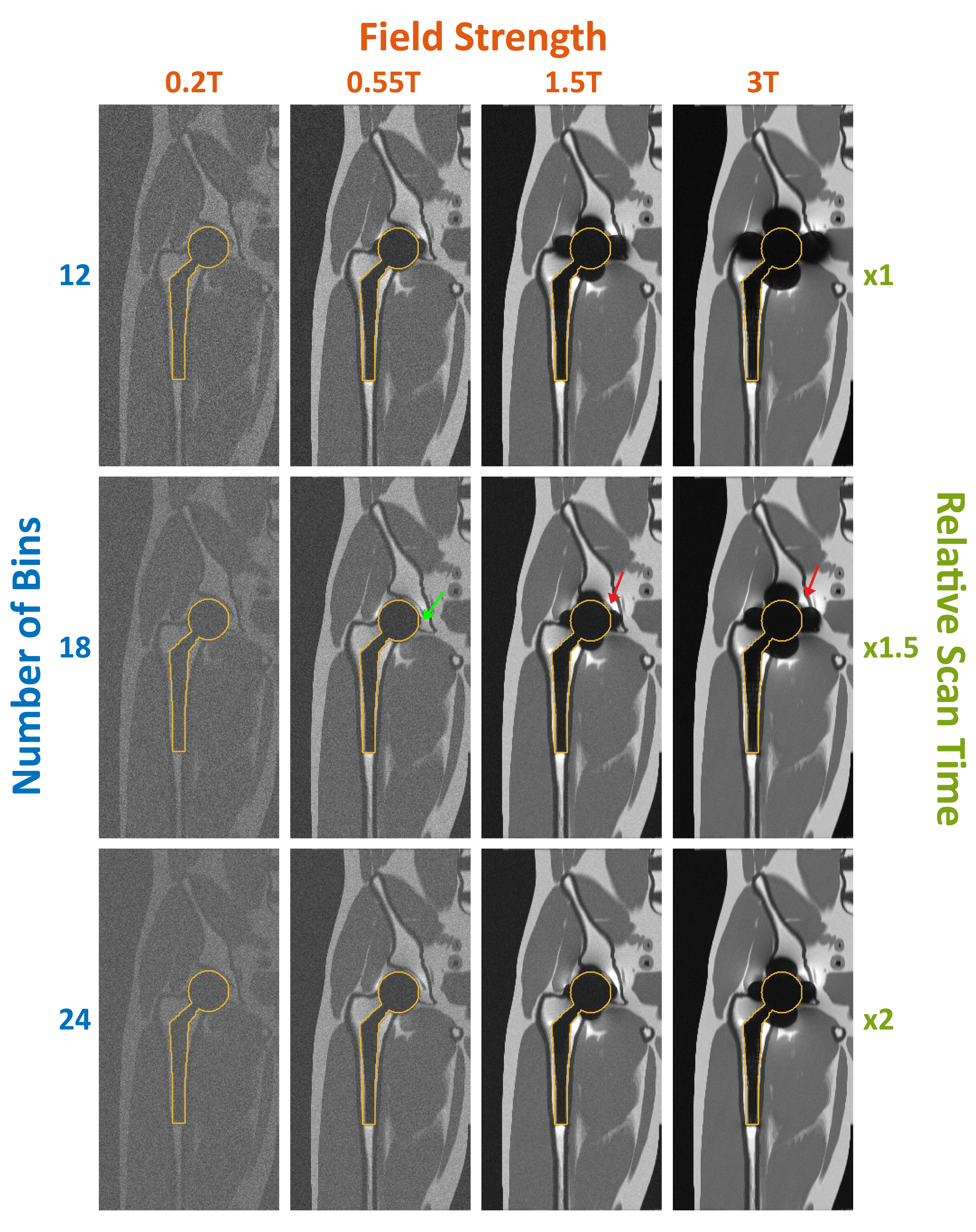
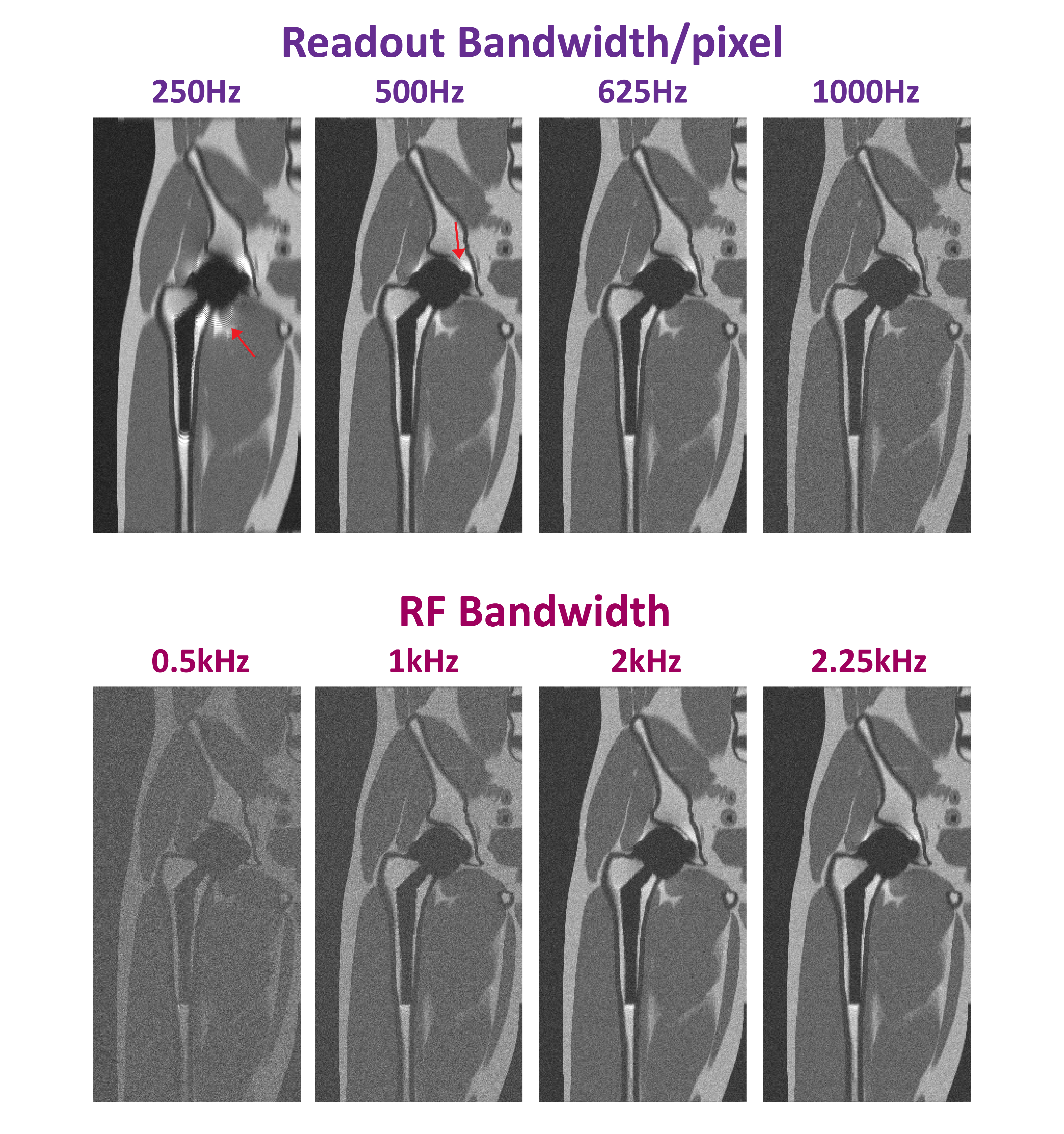
Figure 2 shows a central coronal slice of the simulated MAVRIC-SL volume at different field strengths and with different numbers of spectral bins. All parameters are same except field strength (0.2T,0.55T,1.5T,3T), and total number of spectral bins (12,18,24). As expected, the artifact size decreases for lower field strengths (85,68,48,45 mm at 3T,1.5T,0.55T,0.2T respectively when Nbins=18, and implant diameter=44mm), at the expense of SNR (38.3,19.8,9.2,6.4 dB at 3T,1.5T,0.55T,0.2T respectively when Nbins=18). Notice that extreme frequencies near the metal can be captured with fewer spectral bins at low field.Figure 3 illustrates the effect of readout and RF bandwidth on artifact size and image quality for B0=0.55T, Nbins=12. Simulations are shown with a range of readout bandwidth/pixel (250Hz,500Hz,625Hz,1kHz) when RF bandwidth=2.25kHz (top), and at a range of RF bandwidths (0.5kHz,1kHz,2kHz,2.25kHz) when readout bandwidth/pixel=1kHz (bottom). Everything except the variable parameter is kept same. As readout bandwidth increases, artifact reduces with a corresponding decrease in SNR. As RF bandwidth increases, overlapping of spectral bins, and therefore SNR increases. Wider RF bandwidth can be used safely at 0.55T, as SAR restrictions are relaxed.
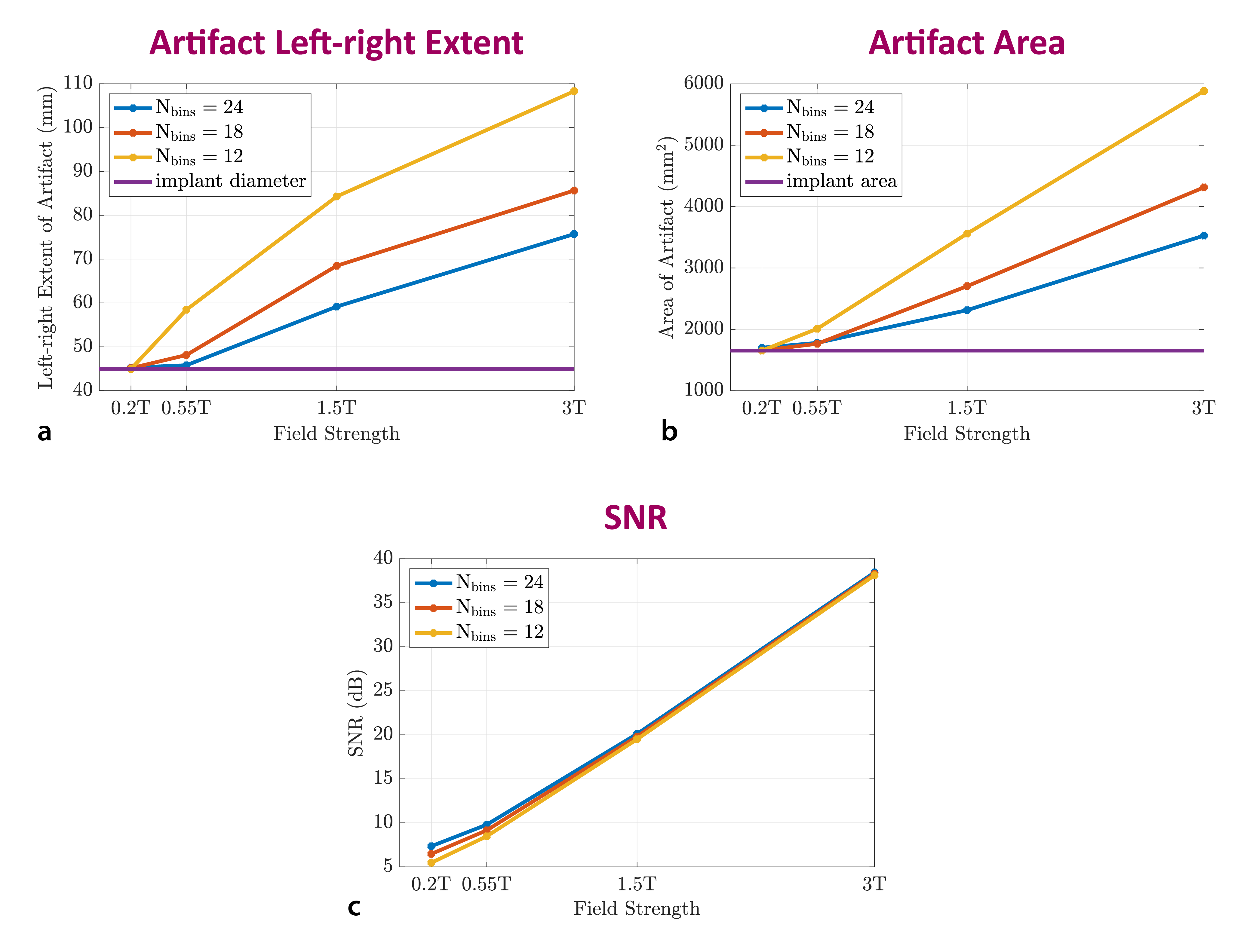
Figure 4 demonstrates the performance of MAVRIC-SL when different Nbins are used at various field strengths. Quantitative metrics such as artifact left-right extent (mm), artifact area (mm2), and SNR (dB) are shown as a function of B0. This analysis can be used to evaluate and find sets of parameters that can give an optimum result for given constraints
DISCUSSION
This simulation framework can be used to anticipate the performance of metal MRI for various field strengths, implant geometries, implant materials, and imaging parameters. It can allow to optimize the protocol beforehand and tailor parameters so that optimum performance can be achieved.We use a single example; one specific body phantom and one specific hip implant, however the pipeline and methodology are general. Our initial simulations suggest that lower field strengths with high-performance gradients could provide better quality metal MSI around THA, compared to what is possible at conventional field strengths, as long as SNR is carefully considered.
CONCLUSION
We have demonstrated a general framework for realistic simulation of metal MSI performance and its dependence on B0 field strength and acquisition parameters. Metal artifacts are significantly reduced at lower field strengths; while number of spectral bins, readout and RF bandwidth can be increased to balance artifact size and SNR.Acknowledgements
KK receives support from a USC Annenberg Graduate Fellowship.References
1. Kremers HM, Larson DR, Crowson CS, et al. Prevalence of Total Hip and Knee Replacement in the United States. J Bone Joint Surg Am. 2015;97(17):1386-1397.
2. Koch KM, Hargreaves BA, Pauly KB, et al. Magnetic Resonance Imaging Near Metal Implants. J Magn Reson Imaging. 2010;32(4):773-787.
3. Segars WP, Sturgeon G, Mendonca S, et al. 4D XCAT phantom for multimodality imaging research. Medical Physics. 2010;37(9):4902-4915.
4. Shi X. MRI near Metal. http://stanford.edu/~xinweis/Software.html.
5. Schenck JF. The role of magnetic susceptibility in magnetic resonance imaging: MRI magnetic compatibility of the first and second kinds. Med Phys. 1996;23(6):815-850.
6. Bottomley PA, Hardy CJ, Argersinger RE, et al. A review of 1H nuclear magnetic resonance relaxation in pathology: Are T1 and T2 diagnostic? Med Phys. 1987;14(1):1-37.
7. Pohmann R, Speck O, Scheffler K. Signal-to-noise ratio and MR tissue parameters in human brain imaging at 3, 7, and 9.4 tesla using current receive coil arrays. Magn Reson Med. 2016;75(2):801-809.
8. Rooney WD, Johnson G, Li X, et al. Magnetic field and tissue dependencies of human brain longitudinal 1H2O relaxation in vivo. Magn Reson Med. 2007;57(2):308-318.
9. Bojorquez JZ, Bricq S, Acquitter C, et al. What are normal relaxation times of tissues at 3 T? Magn Reson Imaging. 2017;35:69-80.
10. Bouwman JG, Bakker CJG. Alias subtraction more efficient than conventional zero-padding in the Fourier-based calculation of the susceptibility induced perturbation of the magnetic field in MR. Magn Reson Med. 2012;68(2):621-630.
11. Koch KM, Brau AC, Chen W, et al. Imaging near metal with a MAVRIC-SEMAC hybrid. Magn Reson Med. 2010;65(1):71-82.
12. Wu Z, Chen W, Nayak KS. Minimum Field Strength Simulator for Proton Density Weighted MRI. PLoS ONE. 2016;11(5): e0154711.
13. Lu W, Pauly KB, Gold GE, et al. SEMAC: slice encoding for metal artifact correction in MRI. Magn Reson Med. 2009;62(1):66-76.
14. Koch KM, Lorbiecki JE, Hinks RS, et al. A multispectral three-dimensional acquisition technique for imaging near metal implants. Magn Reson Med. 2009;61(2):381-390.
Figures