Introduction

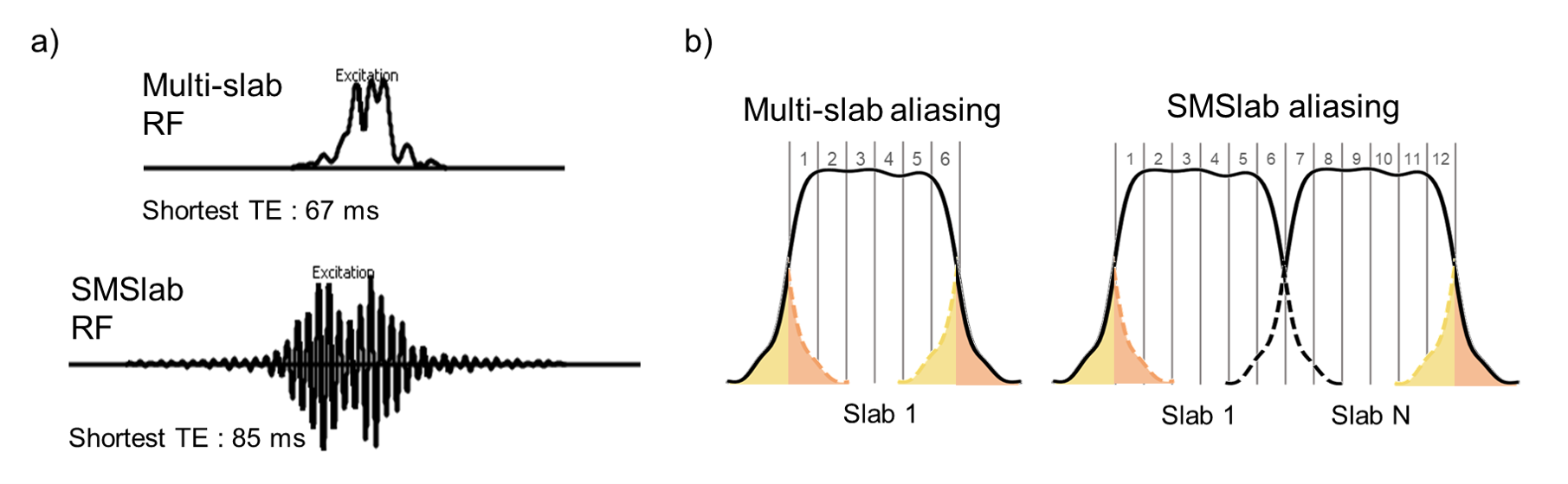
In simultaneous multi-slab (SMSlab) acquisition, multiple 3D slabs are excited simultaneously. It can achieve the optimal signal-to-noise ratio (SNR) efficiency for high-resolution whole-brain diffusion weighted imaging (DWI)¹. However, boundary artifacts restrain its application^2-4. Similar as the boundary artifacts in multi-slab^2,3,5-7, the artifacts manifest as intensity variation and aliasing in the slice direction, which mainly result from the truncated RF pulses. However, in SMSlab, they are more severe. The SMSlab pulses are the summation of multiple pulses, so the pulse durations are prolonged (Fig.1a). The RF pulses have to be further truncated to ensure a short echo time (TE). Moreover, the intra-slab aliasing in multi-slab turns out to be inter-slab aliasing in SMSlab (Fig. 1b).
Nonlinear inversion for slab profile encoding (NPEN)² can solve the boundary artifacts in multi-slab, and it was adapted for SMSlab^1,8. However, its computation is time-consuming, and residual artifacts still exist in the results⁸. Inspired by NPEN, we proposed to reduce the boundary artifacts using a convolutional neural network (CNN) for slab profile encoding (CPEN) in SMSlab.

Methods and materials

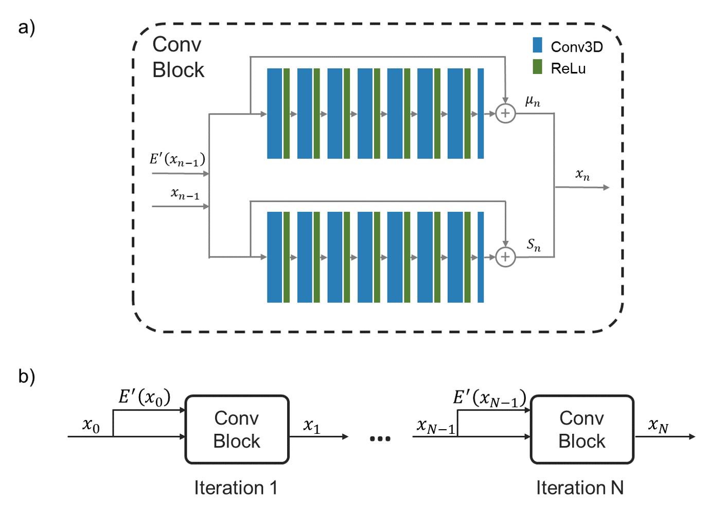
Theory
In image domain, the boundary artifacts in SMSlab can be formulated as Eq. 1. $$ E(x)=A S \mu=I \qquad \qquad [1]$$ $$x=[\mu, S]^{T} \qquad \qquad [2]$$ $$$I$$$ is the image with boundary artifacts; $$$\mu$$$ is the artifact-free image; $$$S$$$ is the concatenation of the slab profiles; $$$A$$$ represents the inter-slab aliasing pattern. The reconstruction is a non-linear inversion problem². If Gauss-Newton algorithm is used, the iteration will be like Eq.3. $$E^{\prime}\left(x_{n-1}\right) \Delta x_{n-1}=I-E\left(x_{n-1}\right) \qquad \qquad [3]$$ $$$E^{\prime}\left(x_{n-1}\right)$$$ is the Fréchet derivate of $$$E\left(x_{n-1}\right)$$$ at the current guess $$$x_{n-1}$$$; $$$\Delta x_{n-1}$$$ is the update at the $$$n$$$th iteration. Rather than solving Eq.3 using least square solution, in CPEN, the optimal solution of $$$\Delta x_{n-1}$$$ is learnt from the training data. As shown in Fig. 2, the unrolled iterative network consists of K repeated CNN blocks. Each block takes $$$E^{\prime}\left(x_{n-1}\right)$$$ and $$$x_{n-1}$$$ as input, and generates $$$x_{n}$$$.
The model is trained with a composite loss function inspired by NPEN². $$\operatorname{loss} =d S S I M+\lambda_{1}\left\|I-E\left(x_{n}\right)\right\|_{2}^{2}+\lambda_{2}\left\|x_{n}-x_{0}\right\|_{2}^{2}+\lambda_{3}\left\|W F \mu_{n}\right\|_{2}^{2}+\lambda_{4} \text {loss}_{\text {smooth}} \qquad \qquad [4]$$ $$$\lambda_{1}$$$, $$$\lambda_{2}$$$, $$$\lambda_{3}$$$ and $$$\lambda_{4}$$$ are the weights of the loss functions. $$$d S S I M$$$ is structural dissimilarity⁹. $$$F$$$ represents fast Fourier transform.$$$W$$$ is a weight matrix with large values at the spike frequencies. $$$\text {loss}_{\text {smooth}}$$$ is the in-plane variance of $$$S_{n}$$$, which constrains the slab profiles to be smooth.

Image acquisition
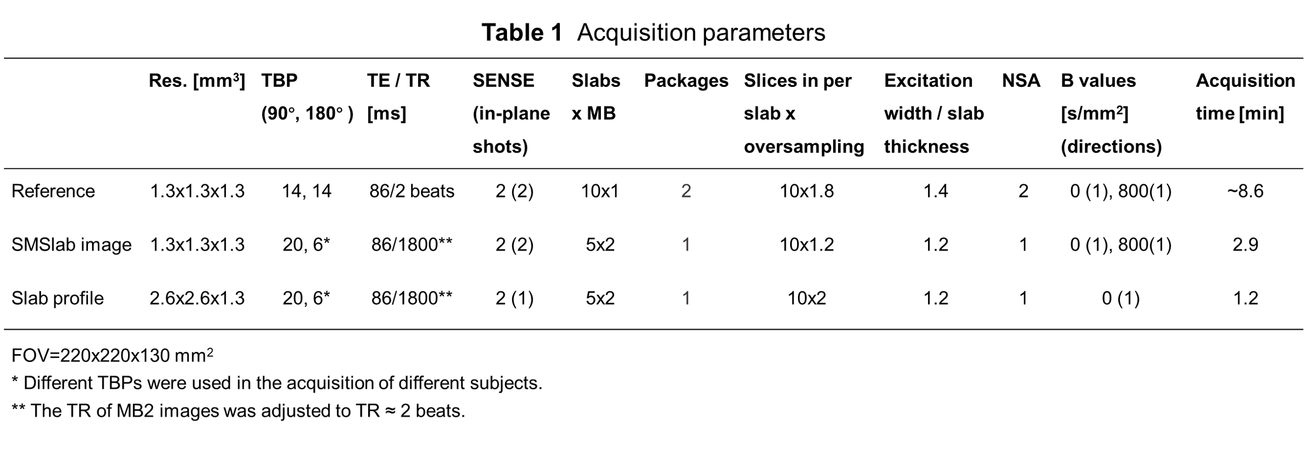
For the training set, images of 9 healthy subjects were acquired with 1.3 mm isotropic resolution. Each acquisition contained reference, SMSlab images and slab profiles. The reference images were acquired with cardiac trigger, and multi-slab was used for RF pulses with higher time-bandwidth-products (TBPs). The TE and repetition time (TR) of the SMSlab images kept the same as those in the reference. Different TBPs were used, so the network could be exposed to different levels of artifacts. The other parameters are listed in Table1.
The model was tested on 3 datasets excluded from the training set. Two of them included reference images. They were acquired with 1.3 mm and 1 mm isotropic resolution, respectively. For the test data, the nominal excitation width of the reference and the SMSlab images were adjusted to ensure comparable SNRs of these two sequences. Another test dataset with 1 mm isotropic resolution consisted of 32 directions. Fractional anisotropy (FA) and mean diffusivity (MD) maps were calculated using FDT from FSL¹⁰. NPEN was also used for comparison.

Results and Discussion

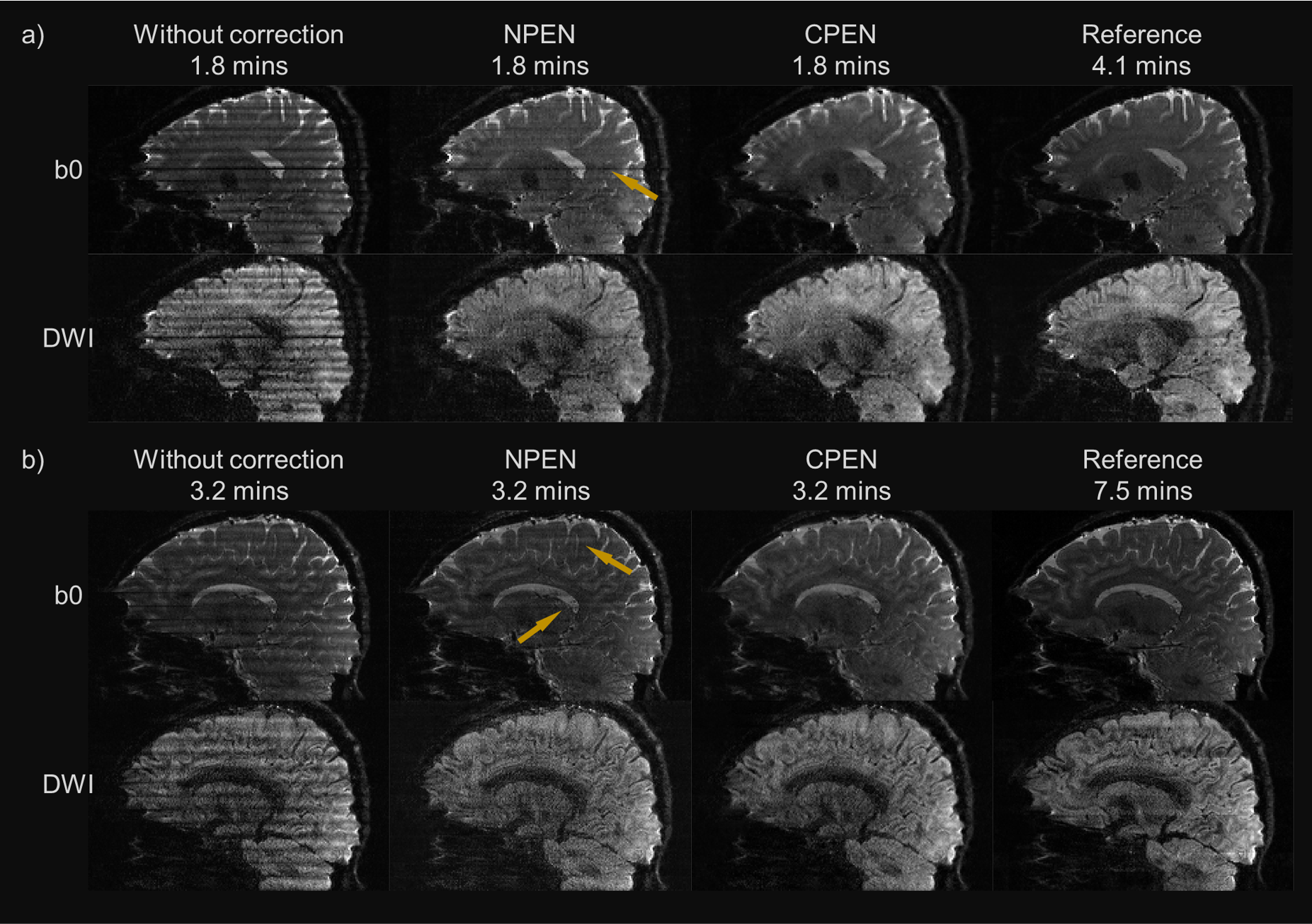
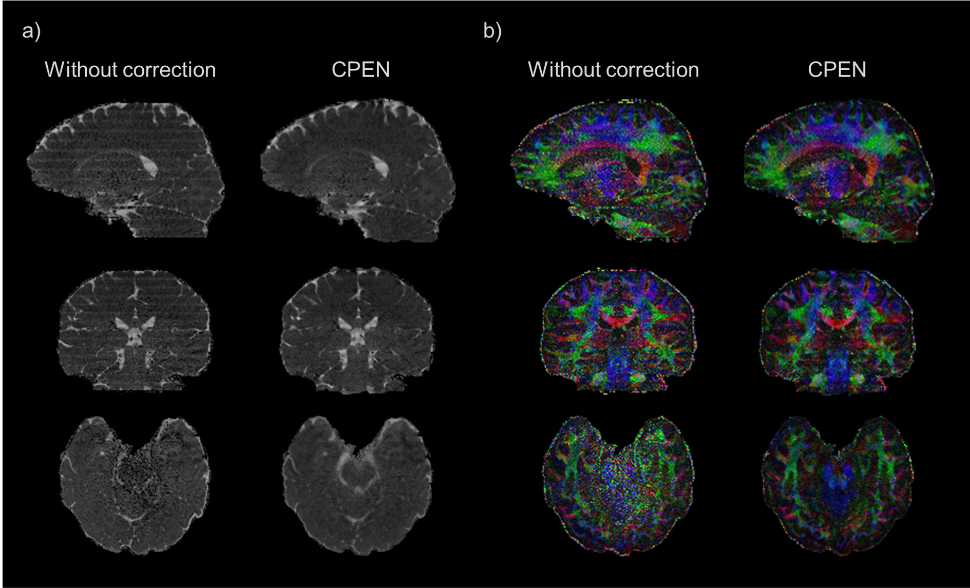
Fig.3 shows the results of test datasets. Residual artifacts (yellow arrows) are visible in SMSlab NPEN. The results of CPEN are more close to the reference images, except for the slight artifacts in the cerebrospinal fluid (CSF) regions, which has little impact on DWI. As for the reference images, the TRs might be inconsistent among different slabs and shots because of the cardiac triggering, so the intensity variation may occur sometimes. The acquisition time of the reference images is more than twice longer than that of the artifact images. That is, using CPEN, small oversampling factors can be used to save the acquisition time. The computation time of 1 volume on CPU is 2 mins and 84 mins for CPEN and NPEN, respectively. CPEN is faster, because it reduces the computational complexity by using single-channel data and used CNN for fast computation.
Fig.4 shows the FA and MD maps of the 32-direction dataset. Without correction, the SNR of the edge slices is so low that the noises in the FA map prevent us from identifying the anatomical structure, and the MD maps also show obvious artifacts. CPEN shows an effective suppression of noise. It significantly increased the SNR of the edge slices.

Conclusion

We proposed a model-based CNN, CPEN, for boundary artifacts correction in SMSlab. CPEN outperforms NPEN in images with different resolutions. CPEN takes advantages of both model-based and data-driven methods. It’s more robust, and its computation is much faster than NPEN. Therefore, CPEN is very promising for boundary artifacts correction in SMSlab, especially when a large number of volumes are acquired. It can also be extended to boundary artifacts correction in multi-slab.

Acknowledgements

No acknowledgement found.