3524
A Method for Correcting Non-linear Errors in Radial Trajectories1MRI Systems Development Department, Canon Medical Systems Corporation, Kanagawa, Japan, 2MRI Systems Development Department, Canon Medical Systems Corporation, Tochigi, Japan, 3Advanced Technology Research Department, Research and Development Center, Canon Medical Systems Corporation, Kanagawa, Japan
Synopsis
The authors propose a new method to use a non-linear model for correcting errors in radial trajectories. The model represents shifts of trajectories as a combination of a linear function and a sigmoid function.
Conventional methods assume that the shifts are proportional to the gradient strengths. However, actual trajectories cannot be represented as linear models precisely due to non-linear imperfections of the gradients such as eddy currents.
The proposed method suppresses streak artifacts and image shadings which appear with conventional linear correction.
Introduction
While radial scans are known as being robust to patient motion, their image quality often suffers from streak artifacts. The reason is that the image quality of radial scans is sensitive to trajectory errors caused by imperfections of gradient fields.To improve image quality, existing methods correct trajectory errors using linear models. The strategies of existing studies include making use of field cameras1, finding the peak of the k-space data2, calculating phase difference from a statistical average3,4, comparing pairs of k-space data in opposite directions5,6, and finding cross-section of trajectories7.
The authors propose a new method to use a non-linear model to correct errors in radial trajectories. The proposed model represents shifts of trajectories as a combination of a linear function and a sigmoid function. The motivation is induced by the insights that actual trajectories cannot be represented as linear models precisely. Imperfections of gradients such as eddy currents are not always linear.
Experimental results show that the proposed method corrects radial trajectories more precisely than the conventional method. In reconstructed images from stack-of-stars scans, the proposed method suppresses streak artifacts which appear with conventional linear correction.
Theory
This section explains how the gradient imperfections cause non-linear trajectory errors. As shown in Figures 2(a) and (b), gradient imperfections cause distortions to the gradient waveforms. Let the ideal gradient waveforms be $$$G^{(i)}_x(t,\theta),\,G^{(i)}_y(t,\theta)$$$ and actual waveforms be $$$G^{(a)}_x(t,\theta),\,G^{(a)}_y(t,\theta)$$$. The former is generated by $$G^{(i)}_x(t,\theta)=G_r(t)\cos\theta,$$ $$G^{(i)}_y(t,\theta)=G_r(t)\sin\theta,$$ where $$$G_r(t)$$$ represents the gradient waveform along the read-out direction. The trajectory $$$(k_x(t,\theta),k_y(t,\theta))$$$ is described as integrals of the actual gradients by $$k_x(t,\theta)=\frac{\gamma}{2\pi}\int_0^tG^{(a)}_x(t,\theta)dt,$$ $$k_y(t,\theta)=\frac{\gamma}{2\pi}\int_0^tG^{(a)}_y(t,\theta)dt.$$ Hence, distorted waveforms result in distortion of the trajectories, as shown in Figure 2(c).Peters et al.4 reported that trajectory errors can be corrected by compensating shifts of the trajectories. The shifts are calculated by $${\Delta}k_x(\theta)=\frac{\gamma}{2\pi}\int_0^{t_c}(G^{(a)}_x(t,\theta)-G^{(i)}_x(t,\theta))dt,$$ $${\Delta}k_y(\theta)=\frac{\gamma}{2\pi}\int_0^{t_c}(G^{(a)}_y(t,\theta)-G^{(i)}_y(t,\theta))dt,$$ where $$$t_c$$$ represents the time of the center of the samplings.
Here, the shifts cannot be assumed to be proportional to $$$(\cos\theta,\sin\theta)$$$ even though the existing studies usually assumed so. Let us suppose gradient delays that have dependency on the gradient strength as $$\tau_x=\tau_{0x}+\tau_{1x}\,G^{(i)}_x(t_c,\theta),$$ $$\tau_y=\tau_{0y}+\tau_{1y}\,G^{(i)}_y(t_c,\theta),$$ where $$$\tau_x,\,\tau_y$$$ represents the delays and $$$\tau_{0x},\,\tau_{0y},\,\tau_{1x},\,\tau_{1y}$$$ are constants. Since $$$(G^{(a)}_x(t,\theta),\,G^{(a)}_y(t,\theta))$$$ can be described as $$G^{(a)}_x(t,\theta)=G^{(i)}_x(t-\tau_x,\theta),$$ $$G^{(a)}_y(t,\theta)=G^{(i)}_y(t-\tau_y,\theta),$$ we obtain $${\Delta}k_x(\theta)=\frac{\gamma}{2\pi}(\tau_{0x}\,G_r(t_c)\,\cos\theta+\frac{\tau_{1x}}{2}\,G_r(t_c)^2\,\cos^2\theta),$$ $${\Delta}k_y(\theta)=\frac{\gamma}{2\pi}(\tau_{0y}\,G_r(t_c)\,\cos\theta+\frac{\tau_{1y}}{2}\,G_r(t_c)^2\,\cos^2\theta).$$ In the equations, 2nd-order dependencies on $$$(\cos\theta,\sin\theta)$$$ are seen. Beyond the example, there can be dependencies of higher order. Therefore, providing an adequate model for the shifts is the target of this study.
Method
The authors propose a non-linear model to predict the correction values. The model is described as $${\Delta}k^{(p)}_x(\theta)=a_x(\cos\theta)+b_x\,\varsigma(c_x\cos\theta),$$ $${\Delta}k^{(p)}_y(\theta)=a_y(\sin\theta)+b_y\,\varsigma(c_y\cos\theta),$$ where $$$a_x,\,b_x,\,c_x,\,a_y,\,b_y,\,c_y$$$ are the model parameters. $$$({\Delta}k^{(p)}_x(\theta),\,{\Delta}k^{(p)}_y(\theta))$$$ represents the predictions of the trajectory shifts to be corrected. $$$\varsigma(\xi)$$$ represents a sigmoid function defined as $$\varsigma(\xi)=\frac{e^\xi-e^{-\xi}}{e^\xi+e^{-\xi}}.$$ Sigmoid function is used to represent the non-linear dependencies.For an evaluation of the non-linear model, the shifts of the trajectories are precisely estimated on a 3T MRI scanner using a cubic phantom. The estimation procedures include acquiring pairs of blades, not pairs of trajectories used conventionally5,6. A blade is a group of parallel trajectories in which additional phase encodings are applied. Figure 3 illustrates the procedure. For each read-out direction, following steps were applied:
(i) Acquire the first blade.
(ii) Acquire the second blade. The second blade is the blade whose direction is opposite to the first blade.
(iii) Apply 2-dimensional Fourier-transformation to the first and second blades.
(iv) Rotate the second transformed data by 180 degrees.
(v) Calculate the difference of the complex phase between the two data.
(vi) Estimate the 2-dimensional slope $$$(\mathit{\Delta}_r,\mathit{\Delta}_p)$$$ of the phase difference.
(vii) Calculate the trajectory shifts from the phase slope by $$\begin{pmatrix}{\Delta}k_x\\{\Delta}k_y\end{pmatrix}=\frac{N_r}{2\pi}\begin{pmatrix}\cos\theta&-\sin\theta\\\sin\theta&\cos\theta\end{pmatrix}\begin{pmatrix}\mathit{\Delta}_r/2\\\mathit{\Delta}_p/2\end{pmatrix}.$$ The model parameters for the non-linear model were determined by fitting to the estimations. Then a root-mean-square error RMSE was calculated to validate the model. For comparison, the RMSE for a linear model5 was also calculated.
For an evaluation of the proposed correction method in actual application, experimental scans were performed on a cubic phantom and the abdomen of a healthy volunteer. Volunteer scanning was conducted under an approved IRB protocol. Golden-angle stack-of-stars trajectories were used in the acquisitions. A gridding algorithm8 was applied in reconstruction, and the trajectory correction was applied by inputting the predicted shifts $$$({\Delta}k^{(p)}_x(\theta),\,{\Delta}k^{(p)}_y(\theta))$$$ into the proposed algorithm. For comparison, reconstruction without correction and reconstruction with a linear correction5 were also performed.
Results
The RMSEs for the result of the conventional linear model and the proposed non-linear model were $$$0.247$$$ and $$$0.067$$$, respectively.Reconstructed images from the phantom scan and the volunteer scan are shown in Figure 4 and 5. The proposed method suppressed streak artifacts and image shading which appeared with conventional linear correction.
Discussion
In the experimental cases, RMSEs and the reconstructed images showed that the proposed method corrects radial trajectories more precisely than a conventional method. These results show that non-linear correction is effective at least on a scanner.The proposed non-linear model is tested on only one scanner. Future work includes testing the effectiveness of the proposed model on other scanners.
Conclusion
The authors propose a new method to use a non-linear model to correct errors in radial trajectories. The proposed method suppresses streak artifacts and image shadings which appear with conventional linear correction.Acknowledgements
No acknowledgement found.References
- Vannesjo SJ, Haeberlin M, Kasper L, et al. Gradient system characterization by impulse response measurements with a dynamic field camera. Magn Reson Med. 2013; 69(2):583–593.
- Smith DS and Welch EB. Self-calibrated gradient delay correction for golden angle radial MRI. Proc. Intl. Soc. Magn. Reson. Med. 2014:1538
- Ahn CB and Cho ZH. A new phase correction method in NMR imaging based on autocorrelation and histogram analysis. IEEE Trans Med Imag. 1987;6(1):32–36
- Peters DC, Derbyshire JA and McVeigh ER. Centering the projection reconstruction trajectory: Reducing gradient delay errors. Magn Reson Med. 2003;50(1):1–6.
- Block KT and Uecker M. Simple Method for Adaptive Gradient-Delay Compensation in Radial MRI. Proc. Intl. Soc. Magn. Reson. Med. 2011:2816
- Moussavi A, Untenberger M, Uecker M and Frahm J. Correction of gradient-induced phase errors in radial MRI. Proc. Intl. Soc. Mag. Reson. Med. 2013:3776
- Rosenzweig S, Holme HCM and Uecker M. Simple Auto-Calibrated Gradient Delay Estimation From Few Spokes Using Radial Intersections (RING). Magn Reson Med. 2019; 81(3):1898-1906
- Jackson JI, Meyer CH, Nishimura DG and Macovski A. Selection of a convolution function for Fourier inversion using gridding [computerised tomography application]. IEEE Trans Med Imag. 1991;10:473-478
Figures
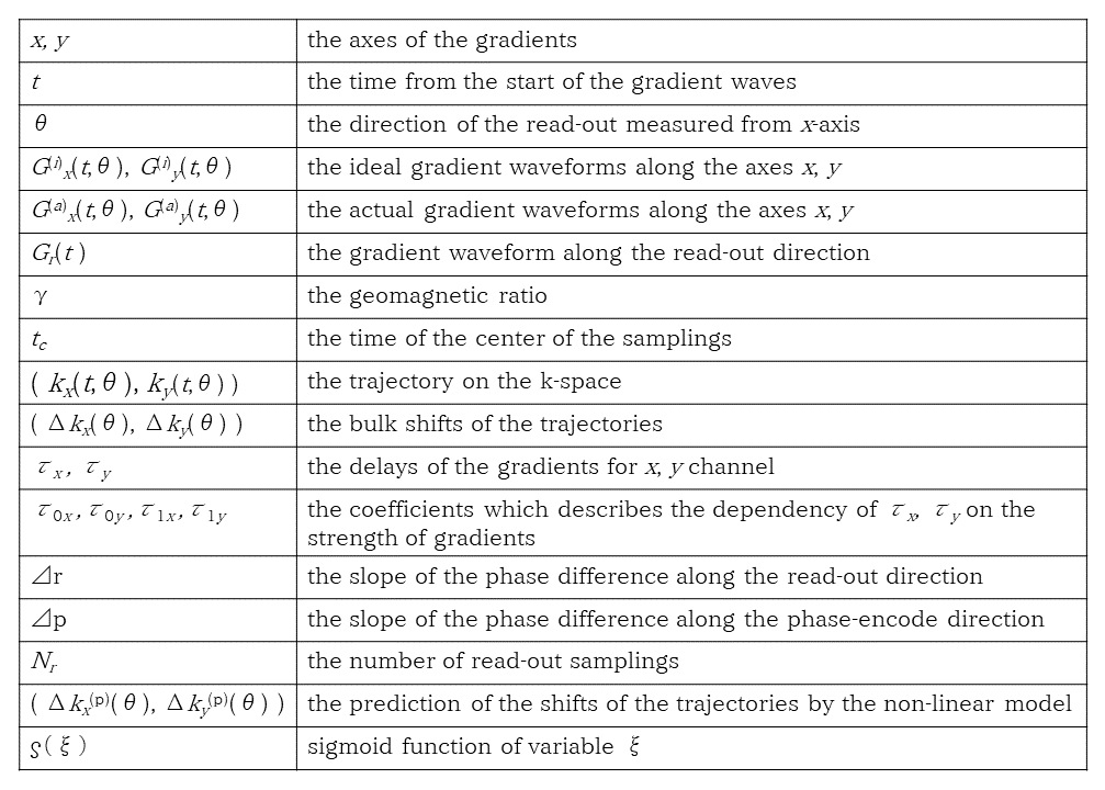
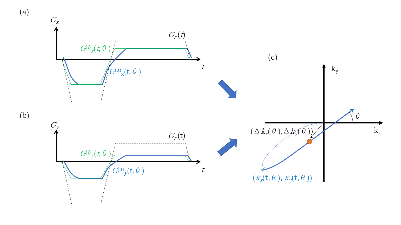
Illustration of relationships between gradient imperfections and radial trajectories
(a) Gradient waveforms along x-axis
(b) Gradient waveforms along y-axis.
Dashed lines represent total gradient along read-out direction.
Green lines represent the ideal waveforms.
Blue lines represent the actual waveforms.
(c) The trajectory on the kx-ky space.
Blue line represents the trajectory.
Orange circle represents the center of the trajectory.
Black arrow represents the shift of the trajectory.
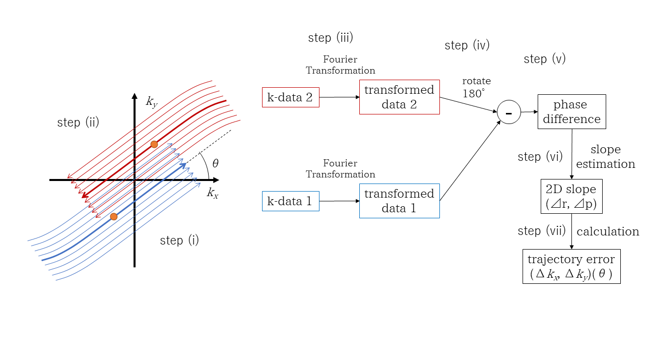
Illustration of the estimation procedure for the trajectory shifts.
Blue arrows represent the first blade.
Red arrows represent the second blade.
Reconstructed images obtained from the stack-of-stars phantom scan
(a) Image reconstructed without correction
(b) Image reconstructed with the linear correction
(c) Image reconstructed with the non-linear correction.
The images at the bottom-left are partial enlarged view of the top-left of the phantom.
The scan parameters: TE=1.3ms, TR=3.6ms, FOV=35cm*35cm, matrix-size=256*256, sampling-pitch=6$$$\mu$$$s, number-of-slices=50, slice-thickness=4mm, number-of-trajectories=200.
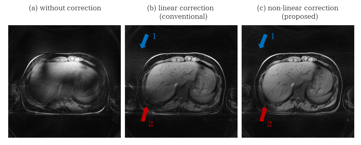
Reconstructed images obtained from the stack-of-stars volunteer scan, under free-breathing
(a) Image reconstructed without correction
(b) Image reconstructed with the linear correction
(c) Image reconstructed with the non-linear correction.
Comparing (b) to (c), streak artifacts (arrow 1) and image shading (arrow 2) are suppressed in (c).
The scan parameters: TE=1.3ms, TR=3.6ms, FOV=35cm*35cm, matrix-size=256*256, sampling-pitch=6$$$\mu$$$s, number-of-slices=50, slice-thickness=4mm, number-of-trajectories=800.