INTRODUCTION

Skull stripping often provides the initial step in neuroimaging pipelines. The accuracy of brain extraction impacts downstream processing steps. Automatic brain extraction procedures are widely used in human neuroimaging^1,2 while extracting brain from preclinical data remains understudied³. We compared the performance of three methods relying on morphological snakes⁵, graph cuts⁴, and convolutional neuronal networks for mouse brain in vivo manganese enhanced MRI (MEMRI).

METHODS

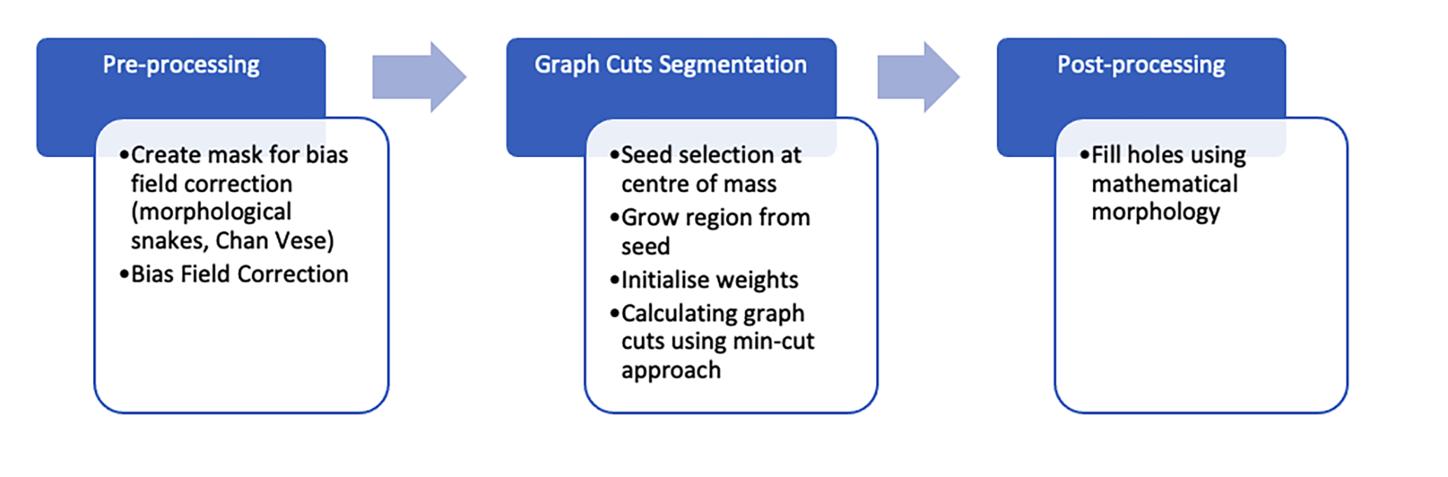
High resolution anatomical images are required for detecting volume changes in mouse models of aging, neurological conditions, or to compare function. We have imaged 33 mice, aged 12-18 months, 8 males, 25 females, of 4 different genotypes: expressing human APOE2 and APOE3 genes, familial Azheimer's disease mutations i.e. APPSwDI/mNos2^−/− and the control mNos2^−/−. In vivo imaging used a 7 T, 20-cm bore Bruker BioSpec, with Avance III console, a 72 mm volume excite coil, and a 4 channel surface receive coil. We used a RARE sequence with TE/TR 25ms/300 ms, 2 NEX, echo separation 6.2 ms, RARE factor 8, BW 100kHz. The image matrix was 200x180x100, and field of view 20x18x10mm. Images were reconstructed at 100µm x100µm x100µm. Manual labels were generated using ITK-SNAP (itksnap.org). We used N4BiasFieldCorrection⁶ with an initial mask generated using morphological snakes, i.e. the Chan-Vese model, implemented in the Scikit-image package⁷ (https://scikit-image.org/). This was seeded in the centre of mass of the image, and allowed to grow.
To produce the final brain segmentation relying on the Chan Vese method we generated 10 instances of morphological active contours without edges, varying the parameters between (4, 0.5), and (0.5, 4), and thresholded the summed results at 90%. Mathematical morphology was used to fill in holes.
For a graph cuts segmentation we adopted the isometric partitioning approach⁴, which cuts narrowly connected regions from the foreground. We chose an initial seed in the centre of mass of the image, assumed to be in the mouse brain, and grew it using a conservative Chan Vese model, chosen so that the initial mask contains only brain voxels. Initial weights between the source (foreground, brain) and image voxels were set to infinity, and between sink (background, non-brain) and image voxels were set to 0. Weights between voxels were initialised in the 6-connected neighbourhood as $$w(i,j)=max(D(vi),D(vj))$$ where D(vi) and D(vj), are distances from vertices to the ROI. Further, we modify weights between voxels so that the cut should be through voxels with low intensity.
Our graph cuts method used the max-flow algorithm⁸ (PyMaxFlow package). We “filled in” remaining holes. The flowchart for this process is shown in Figure 1.
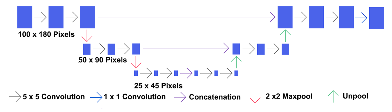
Lastly, we implemented a convolutional neural network (CNN) with a U-net architecture (Figure 2). This relied on TensorFlow 2.3 and consisted of 3 levels of 2 convolutional layers and a down-sampling layer, followed by 3 levels of 2 convolutional layers and an up-sampling layer. Each convolutional layer had a kernel of 5x5, unpadded, and we used rectified linear (ReLU) activation followed by a max-pooling layer to down-sample by 2x2. The final layer consists of a sigmoid activation that predicts whether a pixel belongs to the brain mask class or not. We optimized the model (1,487,169 parameters) using an Adam optimizer with exponential decay learning rate and binary cross entropy as a loss function. We used a leave one out strategy.
The skull stripping algorithms were validated against manually generated masks using Dice and Jaccard indices, sensitivity and specificity. We compared the three methods (active contours, graph cuts, and CNN using one way ANOVA, followed by Tukey post-hoc corrections.

RESULTS

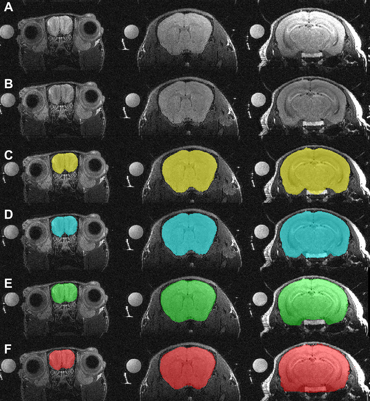
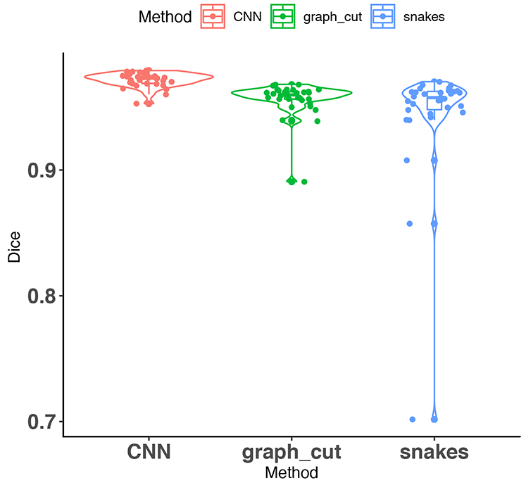
A qualitative comparison of unsupervised segmentation using the Chan Vese, graph cuts, and CNN brain segmentation, relative to the manual masks and the MR images is shown in Figure 3.
A quantitative evaluation of the brain segmentation performance is presented in Figure 4. All methods produced average Dice coefficients > 94%. A one-way ANOVA revealed that differences, though small were significant (F(2,96)=7.135, p=0.001). The post-hoc tests revealed that the U-Net /CNN performed significantly better (0.97 ± 0.01) than the Chan-Vese/snakes model (adjusted p=0.001); and the difference between the U-Net/CNN and the graph cuts approached significance (adjusted p=0.088). The graph cuts approach resulted in Dice scores of 0.96 ± 0.01, while the snakes/Chan-Vese method results were 0.94 ± 0.04, but the difference was not significant.

Discussion

The unsupervised skull stripping methods did not outperform the deep learning approaches, but are fast (~200s using 12 core, AMDRyzen CPU), and can be readily used for preclinical data. The graph cuts method was more stable than the Chan-Vese approach, where some brains were segmented with ~0.70% accuracy. The CNN/U-Net required GPUs for efficient implementation and optimization, and was more time consuming (10 minutes using 4 RTX 8000 NVIDIA GPUs), but more accurate and stable, and thus shows promise for future multi-regional segmentation approaches.

Conclusion

We have implemented three mouse brain segmentation methods for in vivo MEMRI. Unsupervised approaches can be readily incorporated into analysis pipelines, without needing sophisticated computers. The CNN approach was more accurate and more stable, but required training, which benefits from using GPUs. Trained models can be applied to future studies in animal models of neurological conditions, such as Alzheimer’s disease.

Acknowledgements

This work was supported by the National Institutes of Health through R01 AG066184, RF1AG057895, R56 AG05789 and U24 CA220245. The study was also supported by the Research Centre for Informatics, grant number CZ.02.1.01/0.0/16~019/0000765 and by the grant Biomedical data acquisition, processing and visualization, number SGS19/171/OHK3/3T/13.