Introduction

The superior colliculus is a region in the brain stem tectum that has a laminated structure containing seven layers. The depth across the layers is about 4mm, which makes it challenging to observe with magnetic resonance imaging (MRI). Previously, some R2* variations were observed in vivo at 9.4T and assigned to the superficial optic layer (layer III) and the intermediate gray layer (layer IV)¹. In this study, we attempt to validate these observations and further identify layer specific MR properties using post mortem samples measured at high field MRI.

Methods

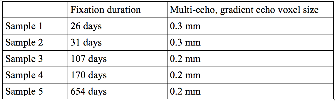
Human brain stem samples (N=5, mean age of subjects: 70y, mean post-mortem interval: 10.7h) were provided by the Institute of Clinical Anatomy and Cell Analysis at the University of Tübingen through the Body Donor program. The donors had no history of neurological disorder. The samples were fixed in formalin with varying duration (Table 1).

The fixed samples were scanned using MRI at 14.1T (Bruker Biospec) using an inversion-recovery MPRAGE (0.3mm isotropic voxel size; FoV=40/33.6/48mm; matrix:133/112/160; TI=25,100,200 400, 600, 1000, 1400, 1800ms; TE/TR=2/2000s; FA=8°; TA=48min for each TI image) for R1 mapping and a multi-echo, gradient echo imaging sequence (0.2mm isotropic voxel size: FoV=42/34.8/36mm, matrix: 210/174/180; TE: from 3ms to 18ms in steps of 3ms; TR=30ms; FA=14°; TA=1h2min38s or 0.3mm isotropic voxel size : FoV=40.4/34.3/48; matrix:134/114/160; TE: from 2.5ms to 15ms in steps of 2.5ms; TR=20ms; FA=10°; TA=5min39s) for R2* mapping.

R1 maps were obtained using a 3-parameter fit that included the inversion efficiency. The sign of the first magnitude data-points was inverted and fitting was performed twice, with different signs of the minimum magnitude value. The parameters that yielded the smallest covariance of the residuals were chosen and the R1-value selected for the final map. R2* maps were obtained by fitting the square of the magnitude intensities. Both R1 and R2* were fitted using a Levenberg-Marquardt non-linear regression algorithm with steepest gradient descent. The maps with 0.3mm voxel-sizes were resampled to 0.2mm using nearest neighbour interpolation.

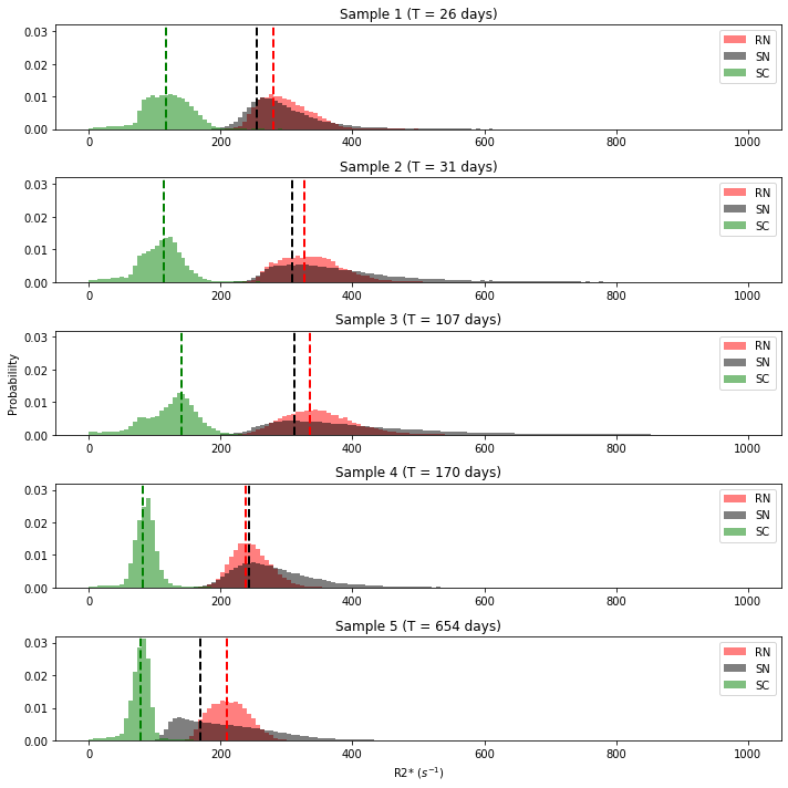
To investigate R2* changes during storage in formalin, we selected three regions of interest (ROIs): superior colliculus, red nucleus and substantia nigra. The ROIs were segmented using ITKsnap.

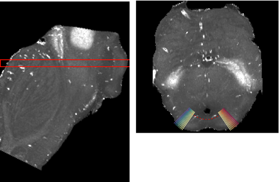
For superior colliculus depth analysis, we fit a second order polynomial to the boundary between the periaqueductal gray and the superior colliculus. We generated vectors orthogonally to the polynomial. R1 and R2* values were extracted along each vector (Figure 1). For sample 3, only one hemisphere was used. Voxels with R2* values over 200 s^-1 were excluded.

Results

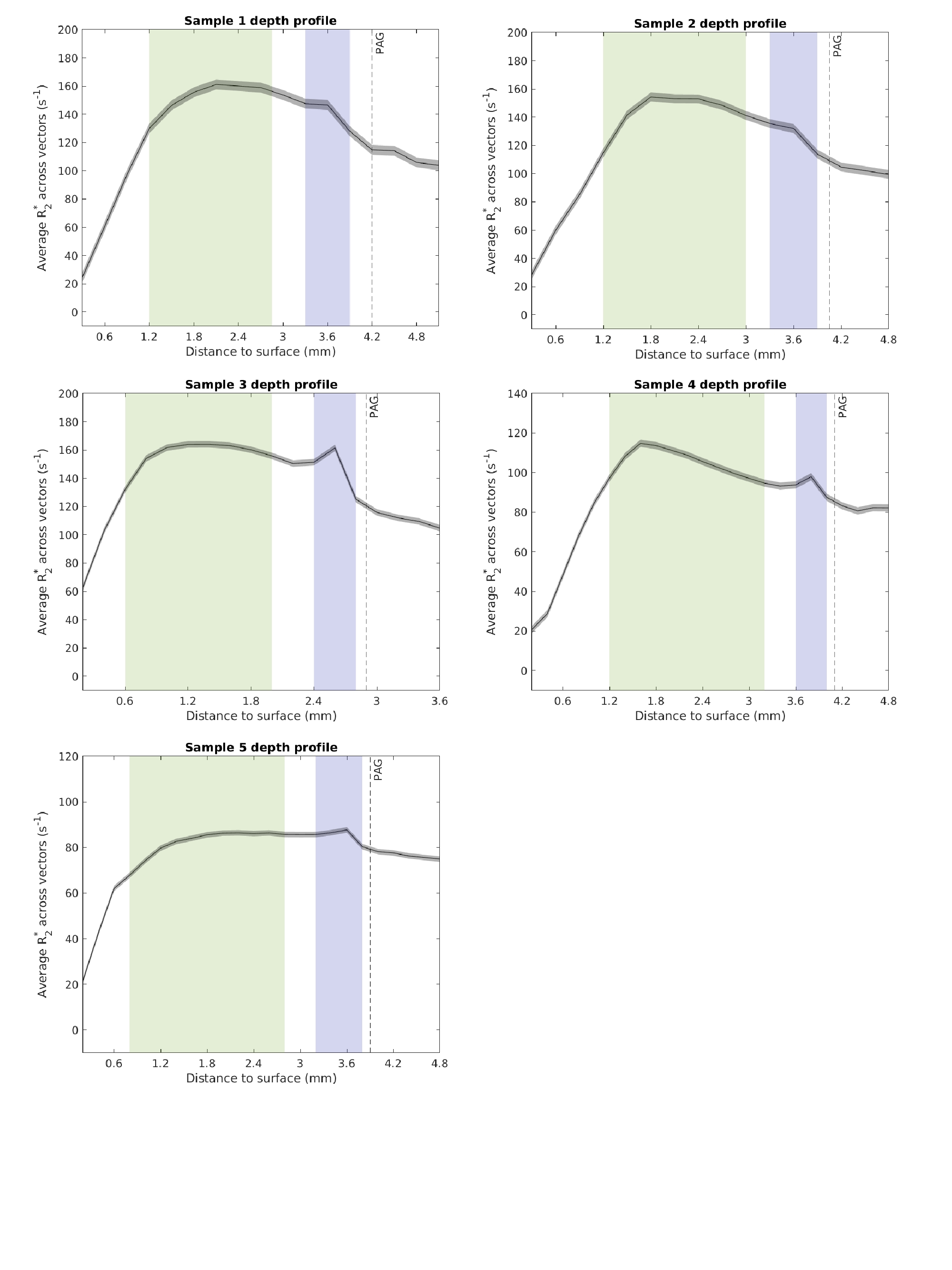
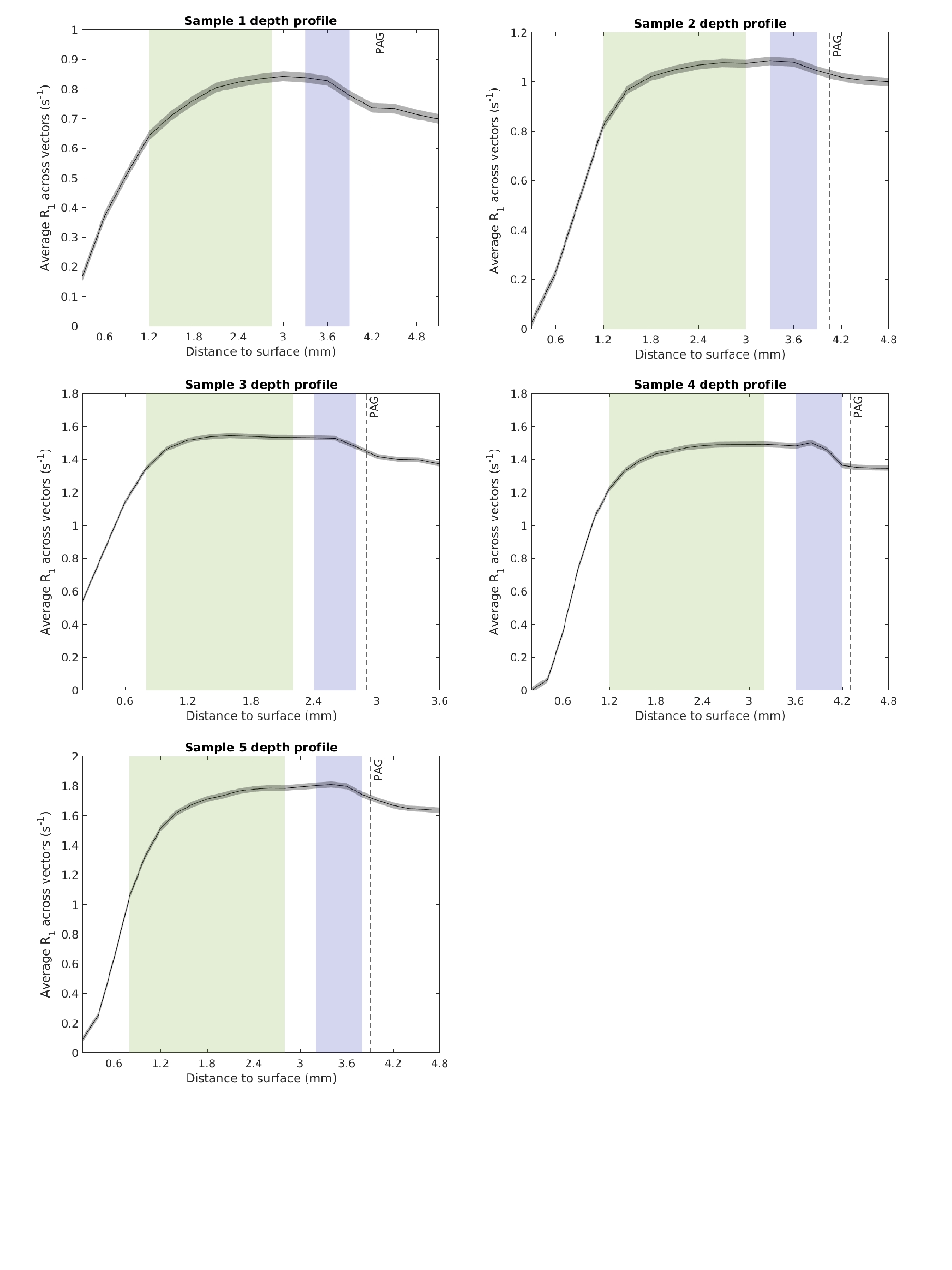
Figure 2 shows the histogram of R2* within the ROIs for each sample. There is a drastic decrease in R2* after at least 5 months. Despite prolonged storage, some features were still discernible. Notably increased R2* and R1 values were observed in a deep layer in immediate proximity with the periaqueductal gray (Figure 3 and 4). This peak resulted even more clear in samples measured with 0.2mm voxel size (R2* of sample 3, 4 and 5). In R2*, maxima located in the intermediate layer were observed except for sample 5. The decrease of R2* in sample 5 could be due to long storage in formalin (22 months). In line with the in vivo study, R1 didn’t show much variation between the layers of superior colliculus¹, but ex vivo a strong difference in R1 between the periaqueductal gray and the deepest colliculus layer was observed.

Discussion

The ROIs showed an R2* decrease already after 5 months of fixation. A decrease in R2* may occur through loss of iron from tissue to the formalin solution. Previously, iron leakage from the brain tissue to the formalin solution has been observed after several years of storage^2,3.

In these ex vivo samples we found no evidence of an increased R2* in the intermediate gray layer. The maximum peaks in the R2* map likely correspond to two layers in the superior colliculus containing myelinated axons: the superficial optic layer (layer III) and the deep white layer (layer VII). While the first layer could be observed in vivo, the deep white layer has not been observed previously¹. This could be due to the coarser spatial sampling used in vivo with 0.4mm voxel-sizes. Indeed, ex vivo we found that detection of this layer was facilitated with 0.2mm voxel-sizes.

In this study, we didn’t cover the entire superior colliculus, only the middle planes where the superior colliculus depth was thickest. In order to include the whole superior colliculus for depth analysis, 3 dimensional analysis covering the entire rostro-caudal axis should be used.

Conclusion

In this study, we investigated layer specific MR properties in the superior colliculus by measuring post mortem human brain stem samples at high-field. There was an overall decrease of R2* when the samples were stored in formalin already after 5 months. Similar to in vivo, the R2* was increased in an area likely corresponding to layer III. For the first time we also report an increase in R2* in proximity to the border of the periaqueductal gray, likely corresponding to layer VII of the superior colliculus.

Acknowledgements

No acknowledgement found.