Introduction

With the advancement of ultra-high performance gradient coil technology, peripheral nerve stimulation (PNS) has become an increasingly important safety consideration in MRI scanning, which impacts gradient design constraints [1]. PNS in MRI arises from rapid transitions of current waveforms in a gradient coil that generate time-varying magnetic fields in space. These fields, in turn, generate electric fields in the body that may stimulate peripheral nerves. The equivalence between magnetic stimulation and electric stimulation has been discussed extensively. It has been previously reported and debated that the chronaxie time $$$\tau_c$$$ of PNS response in the arm from the magnetic stimulation (MS) by a figure-8 coil is different with that from the electric stimulation (ES) by a pair of electrodes [2,3]. Subsequent experiments confirmed the difference but definitive explanations for this observation have not yet to be made [4]. On the other hand, electromagnetic simulations and neurodynamic simulations for both cases haven’t been well compared. In this study, we simulated the electric fields along the nerve induced by MS and ES and found that the field intensity profile from the two cases are indeed very different and PNS initiation locations are consistent with the experiment results in literature, but chronaxie values in both cases are not as different as those in [2,4].

Method

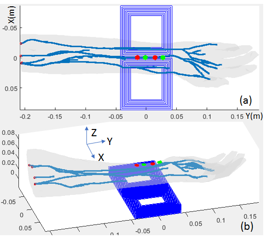
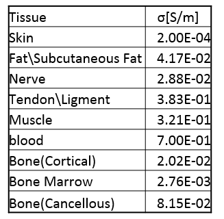
The positions of the electrodes for ES and the figure-8 coil for MS are illustrated in Fig.1(a) and (b) (rendered in the same picture). According to Recoskie, et al., [2], for ES, the electrodes were placed on the distal, anterior surface of the forearm with a separation of 2.9 cm. Different voltages were assigned to the two electrodes to establish the electric field. For MS, each coil set of the figure-8 coil pair was composed of 9x9 square turns, with the inner edge length=5 cm, outer edge length=8.7 cm, and total coil thickness ~2 cm. The coil was positioned underneath the arm model, with the center in the x-y plane aligned to the electrode position. The electric fields in both cases are simulated on the Yoon-sun arm model (IT’IS foundation, Zurich, Switzerland) with the quasi-static solver in Sim4Life (Zurich Med Tech, Zurich, Switzerland) at an arbitrary 1000 Hz with a 1x1x1$$$m^3$$$ mesh grid. The electric conductivity of tissues can be found in Table.1. The electric field was further used for the neurodynamic simulation to find the action potential initiation positions on nerve trajectories. The neurodynamic simulation was performed in NEURON (Yale University, New Haven, CT) which was integrated in Sim4Life. Axion utilized MRG model[6] with fiber diameter set to 16um for motor nerves.

Results and Discussions

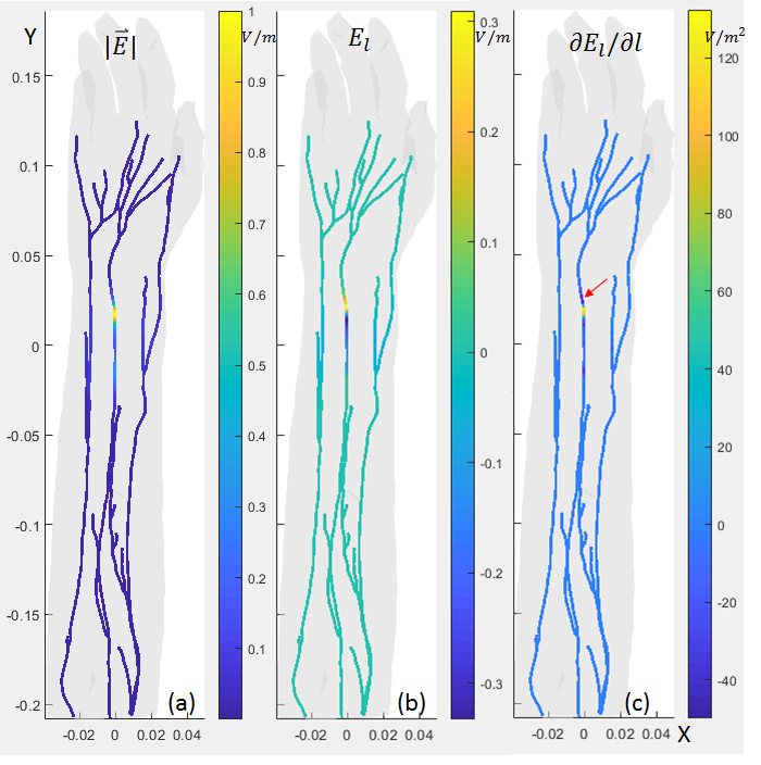
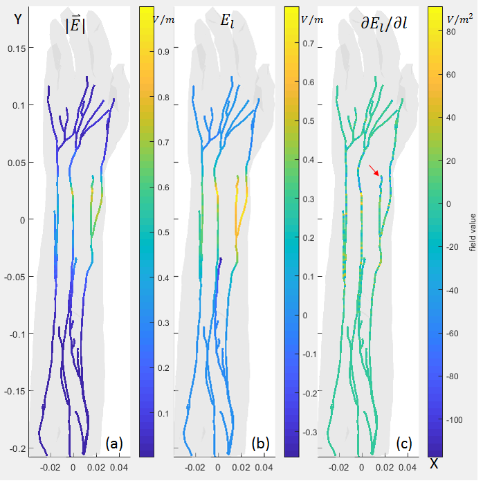
Fig.2(a) and Fig.3(a) show the electric field amplitude $$$|\vec{E}|$$$ on the nerve trajectories for ES and MS, respectively. It can be seen that in ES situation, the E-field with large field values were only distributed in locations very close the electrodes. The E-field decays rapidly such that only part of the nerve under the electrodes was affected. In comparison, in the MS case, the E-field is more evenly distributed and peak values appear on several nerve trajectories. Fig.2(b) and Fig.3(b) show $$$E_l$$$, the E-field component that projected to the tangential direction of the nerve trajectories. $$$E_l$$$ distribution is similar to $$$|\vec{E}|$$$.

Fig.2(c) and Fig.3(c) show the $$$\partial{E_l}/\partial{l}$$$ (Activating Function, AF [5]) on the nerves. AF is more direct to nerve stimulation. Local sharp bends or abrupt termination of the nerve trajectory might result in a larger AF and lower PNS thresholds. From the plots, AF is distributed more randomly for both cases due to the nerve trajectory profile and the local tissue electric-conductivity. But for ES case, the high values were still very close the electrode. This is consistent with the observation in [2], that for ES, all subjects reported the primary location of the sensations to be directly underneath the electrodes, but for MS, subjects reported sensations at many different locations.

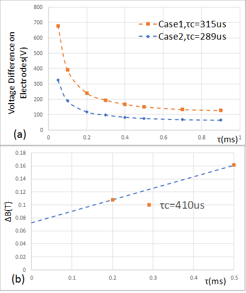
Neurodynamic simulation for both ES and MS cases were performed. It was found that move the electrode closer to the nerve might lower down the rheobase (by using electrode voltage) but only change the chronaxie a little (refer to Fig.4). Rheobase calculated by Case 2 is relatively closer to, but generally higher than that in [2,4], probably due to the discrepancy of the tissue property between the simulation and real situation. The chronaxie calculated from ES and MS with MRG model has some difference, but still at the same order of magnitude. According to [4], chronaxie time values in the range from ~50us to ~400us have been reported from different sources, further investigation is still needed to address the big differences on chronaxie by experiments in [2,4].

Conclusion

Electromagnetic simulations and neurodynamic simulations have been performed for the Yoon-sun arm model. It was found that $$$|\vec{E}|$$$,$$$E_l$$$ and $$$\partial{E_l}/\partial{l}$$$ profiles and the PNS initiation locations for ES and MS cases are very different. Neurodynamic simulation didn’t find big difference on chronaxie between ES and MS situations with with MRG axion model and Yoon-sun anatomical arm model.

Acknowledgements

The work was supported in part by NIH R01EB010065 and U01EB02445