3431
Gaussian Mixture for Peak Identification in Non-Negative Least Squares Fitting of the IVIM Signal1InBrain Lab - University of Sao Paulo, Ribeirao Preto, Brazil, 2LIM44, Instituto e Departamento de Radiologia, Faculdade de Medicina, Universidade de Sao Paulo, Sao Paulo, Brazil
Synopsis
The analysis of the Intravoxel Incoherent Motion (IVIM) signal can be performed with the Non-Negative Least Squares (NNLS) method. It allows detecting an indeterminate number of peaks associated with the multiple exponentials that compose the IVIM signal. Thus, it becomes essential to identify and classify these peaks. We performed a new method to analyze the NNLS spectrum applying the Gaussian Mixture. We obtained pseudo-diffusion maps with better contrast to visualize gliomas. Gaussian Mixture seems to replace the traditional peak search and classification algorithms, opening up possibilities to explore the NNLS spectrum.
Introduction
Intravoxel Incoherent Motion (IVIM) is used to analyze microvascular perfusion by exploring a scaling in diffusion weighting. The signal is modeled in terms of the acquired b-values. The technique and the bi-exponential model of signal interpretation were introduced in 1986 by Denis Le Bihan1.$$\frac{S_{b}}{S_{0}}=(1-f)e^{-bD} +fe^{-bD^{*}}$$
D is the diffusion coefficient, D* is the pseudo-diffusion coefficient, and f is the perfusion fraction. A good fit of the curve is essential for the IVIM application, so the problem of multiple exponentials has been explored in MRI and NMR2. Among the fitting methods, Non-Negative Least Squares (NNLS)3 stands out for not assuming a certain amount of exponentials, not needing initial conditions, and being a single-step method. When applying the NNLS, we minimize the error associated with equation 2, where M is the number of compartments, and i are the observations.
$$S(b_{i})=\sum^{M}_{j=1}{s(D_{j})e^{-b_{i}D_{j}}}$$
Gaussian Mixture Modeling consists of a probabilistic method to deal with the Fuzzy clustering problem, to characterize i observations in k groups. The method assumes that the data was obtained by k gaussians and then maximizes the likelihood value using an Expectation Maximization (EM) algorithm4.
$$p(\chi_{i}|\theta)=\sum^{k}_{j=1}{\pi_{j}N(\chi_{i}|\mu_{j},\sum_{j})}$$
πj is the mixing ratio, $$$N(\chi_{i}|\mu_{j},\sum_{j})$$$ is the Gaussian curve with mean μj and covariance matrix ∑j. The Gaussian Mixture used to identify peaks implies making these peaks discrete in continuous curves, which allows the best identification and opens up possibilities to explore the NNLS spectrum as multi-compartment models of IVIM5.
Methods
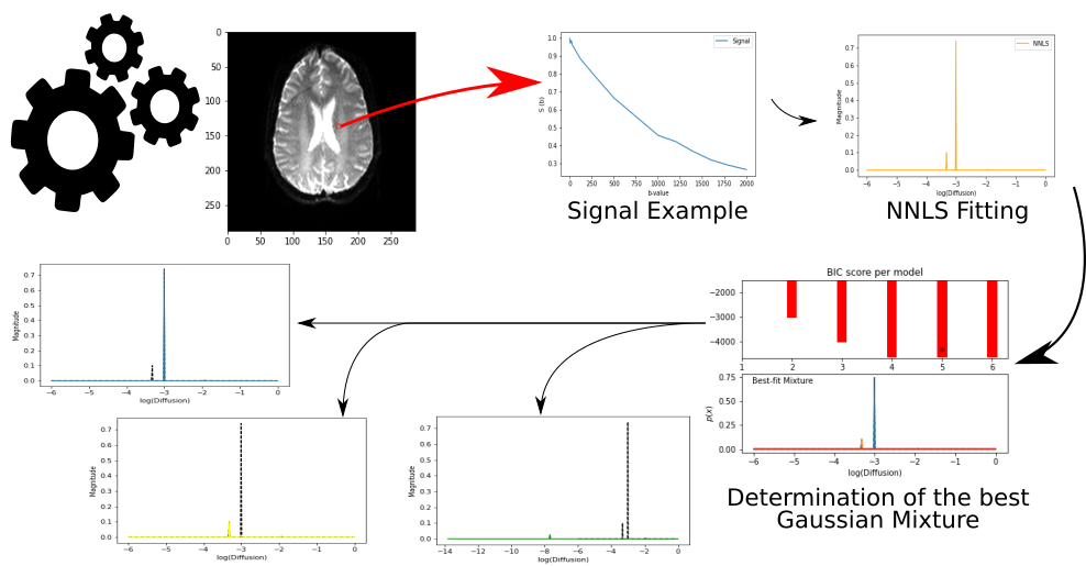
In a 3T MRI system, IVIM images were acquired with 15 b-values (0, 4, 8, 16, 30, 60, 120, 250, 500, 1000, 1200, 1400, 1600, 1800, 2000 s/mm²), 20 slices, and voxel size of 0.83x0.83x5 mm³. Images were preprocessed in SPM12 to correct head-movement artifacts and leakage currents and register with high-resolution T1-weighted images.We used 400 compartments6 in the field of diffusion for the NNLS fitting. The Gaussian Mixture implementation implies a Gaussian curve of probability associated with each peak that fits the ideal number of peaks through the Bayesian Information Criterion (BIC) that is a statistical criterion for model selection. For the processing of these images, we used SPM12 and scripts developed in Python with the libraries Nibabel, Dipy, Numpy, and Scikit-learn. Figure 1 shows the processing scheme.
Diffusion, pseudo-diffusion, and perfusion fraction maps of one healthy individual and two patients with glioma were obtained using the Gaussian Mixture and the traditional algorithm to find a peak. The latter checks if the value at the point is greater than its neighbors.
Results
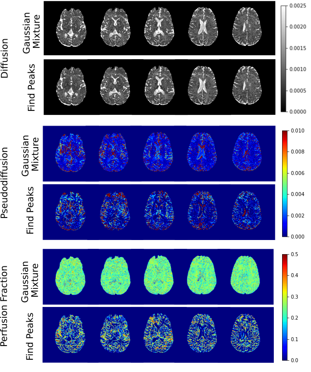
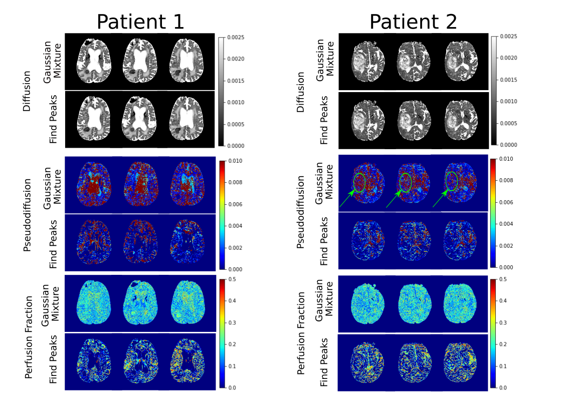
Figure 2 shows the results for the healthy subject. Average values for D, D*, and f were (10 ± 100 ) x 10-3 mm2/s, (200 ± 300) x 10-3 mm2/s, and 0.2 ± 0.1 when applying the Gaussian Mixture. Without using the Gaussian Mixture, average values were: (3 ± 20) x 10-3 mm2/s, (20 ± 100) x 10-3 mm2/s, and 0.3 ± 0.2. For both methods, diffusion values were in the same order; however, for Gaussian Mixture, a higher pseudo-diffusion mean value was observed, although there are little discrepancies in the contrast pattern. Figure 3 shows three slices of each patient. We can observe the glioma through the diffusion images. Pseudo-diffusion maps obtained with the Gaussian Mixture showed better contrast for the glioma identification than the traditional peak-search method. On the other hand, perfusion fraction maps were obtained with lower contrast-to-noise ratio.Discussion
We observed qualitative similarity between the diffusion and pseudo-diffusion maps of the healthy individual. However, a discrepancy of the Gaussian Mixture’s pseudo-diffusion average values is probably due to the misclassification of the peaks. For patients with glioma, pseudo-diffusion maps obtained with the Gaussian Mixture showed better contrast to visualize the tumors. Therefore, through this method, we can be more confident that the peak found is not noise. Our next step is to analyze a set of images from twenty healthy individuals and twenty patients with glioma to check the method’s consistency and improve the fitting with the Gaussian Mixture.Conclusion
We can conclude that the Gaussian Mixture method is an alternative to replace the traditional peak search and classification algorithms. Its use for identifying the peaks opens up several possibilities to explore the NNLS spectrum, from the analysis of the area under the curve to a better understanding of the probability density functions that compose the spectrum.Acknowledgements
CNPq - process number 151245/2019-3. FAPESP - process number 2019/06148-6. FAPESP - process number 2018/11881-1.References
1. D. Le Bihan et al. MR imaging of intravoxel incoherent motions: application to diffusion and perfusion in neurologic disorders. In: Radiology 161.2 (1986), pp. 401–407. doi: 10.1148/radiology.161.182.3763909.
2. Raj A, Pandya S, Shen X, LoCastro E, Nguyen TD, Gauthier SA. Multi-compartment T2 relaxometry using a spatially constrained multi-Gaussian model. PLoS One. 2014;9(6):e98391. Published 2014 Jun 4. doi:10.1371/journal.pone.0098391
3. Lawson, Charles L., and Richard J. Hanson. Solving least squares problems. Society for Industrial and Applied Mathematics, 1995.
4. Reynolds, Douglas A. "Gaussian Mixture Models." Encyclopedia of biometrics 741 (2009).
5. Cercueil, JP., Petit, JM., Nougaret, S. et al. Intravoxel incoherent motion diffusion-weighted imaging in the liver: comparison of mono-, bi- and tri-exponential modeling at 3.0-T. Eur Radiol 25, 1541–1550 (2015). https://doi.org/10.1007/s00330-014-3554-6.
6. Paschoal, A. M. (2019). Optimization and application of quantitative magnetic resonance imaging methods to analyze brain perfusion and function. Doctoral Thesis, Faculdade de Filosofia, Ciências e Letras de Ribeirão Preto, University of São Paulo, Ribeirão Preto. doi:10.11606/T.59.2020.tde-19032020-104417. Retrieved 2020-12-13, from www.teses.usp.br.
Figures