3422
Feasibility of white matter Standard Model parameter estimation in clinical settings1Radiology, NYU School of Medicine, New York, NY, United States
Synopsis
Robust parameter estimation of the Standard Model (SM) for diffusion in white matter has been elusive due to intrinsic model degeneracies and insufficient measurements. To design optimal scanner-specific protocols, we couple multidimensional protocol optimization for estimation of microstructural tissue properties in 15 minute acquisitions on clinical scanners with varying gradient performance. We show reproducible scan-rescan results and assess inter-scanner variability ranging from 1 to 8% depending on parameters. Results suggest that combining denoising, protocol optimization, and robust parameter estimation may enable quantitative microstructure mapping in clinical settings.
Introduction
The driving force for developing biophysical models of diffusion MRI (dMRI) is increased microstructural specificity to pathological changes. In brain white matter (WM), the Standard Model (SM)1 has been widely adopted. However, for single pulsed-field gradient dMRI acquisitions, unconstrained estimation of SM parameters is ill-conditioned unless strong diffusion weightings or orthogonal measurements are acquired2,3,4,5,6. Here we optimize and evaluate a multidimensional dMRI protocol for SM estimation in 15 minutes using both linear and non-linear tensor encoding acquisitions7,8. As additional incentive, we aim to achieve this on clinical scanners with varying gradient specifications and evaluate scan-rescan variability accross different scanners and protocols.Theory
Multidimensional dMRI measurements are represented by a rank-2 symmetric b-tensor $$$B_{ij}=b(b_\Delta n_in_j+\frac{1-b_\Delta}{3}\delta_{ij})$$$, where $$$\mathbf{\hat{n}}$$$ defines tensor orientation and $$$b_\Delta$$$ tensor shape, e.g. $$$b_\Delta=1$$$ for linear or $$$b_\Delta=0$$$ for spherical encoding, $$$b$$$ the diffusion weighting (i.e. size).The Standard Model signal is the convolution over the unit sphere9 of the fibers' orientation distribution function (ODF) $$$\mathcal{P}(\hat{\mathbf{u}})$$$ and the response signal of a fiber segment $$$\mathcal{K}(\boldsymbol{B},\hat{\mathbf{u}})$$$
$$S(\boldsymbol{B})=S_0 \int_{\mathbb{S}^2}\mathcal{P}(\hat{\mathbf{u}})\mathcal{K}(\boldsymbol{B},\hat{\mathbf{u}})\,dS_{\hat{\mathbf{u}}},$$where $$$S_0\equiv S(\boldsymbol{B})|_{\boldsymbol{B}=0}$$$ is the non-weighted diffusion signal, and$$\mathcal{K}(\boldsymbol{B},\hat{\mathbf{u}})=f\exp\bigl[- D_{\text{a}}B_{ij}u_iu_j\bigr]+(1-f-f_\text{FW})\exp\bigl[-bD_\text{e}^\perp -(D_\text{e}^\parallel-D_\text{e}^\perp)B_{ij}u_iu_j\bigr]+f_\text{FW}\exp\bigl[-bD_\text{FW}\bigr]$$with $$$\hat{\mathbf{u}}$$$ the fiber orientation, acquired with the b-tensor $$$\boldsymbol{B}$$$ (Einstein's summation notation assumed). $$$f$$$ and $$$f_\text{FW}$$$ are the $$$T_2$$$-weighted intra-axonal and free-water signal fractions, and $$$D_{\text{a}}$$$, $$$D_\text{e}^\parallel$$$,$$$D_\text{e}^\perp$$$, and $$$D_\text{FW}$$$, the axial intra-axonal, axial extra-axonal, radial extra-axonal, and free-water diffusivities, respectively19.
Methods
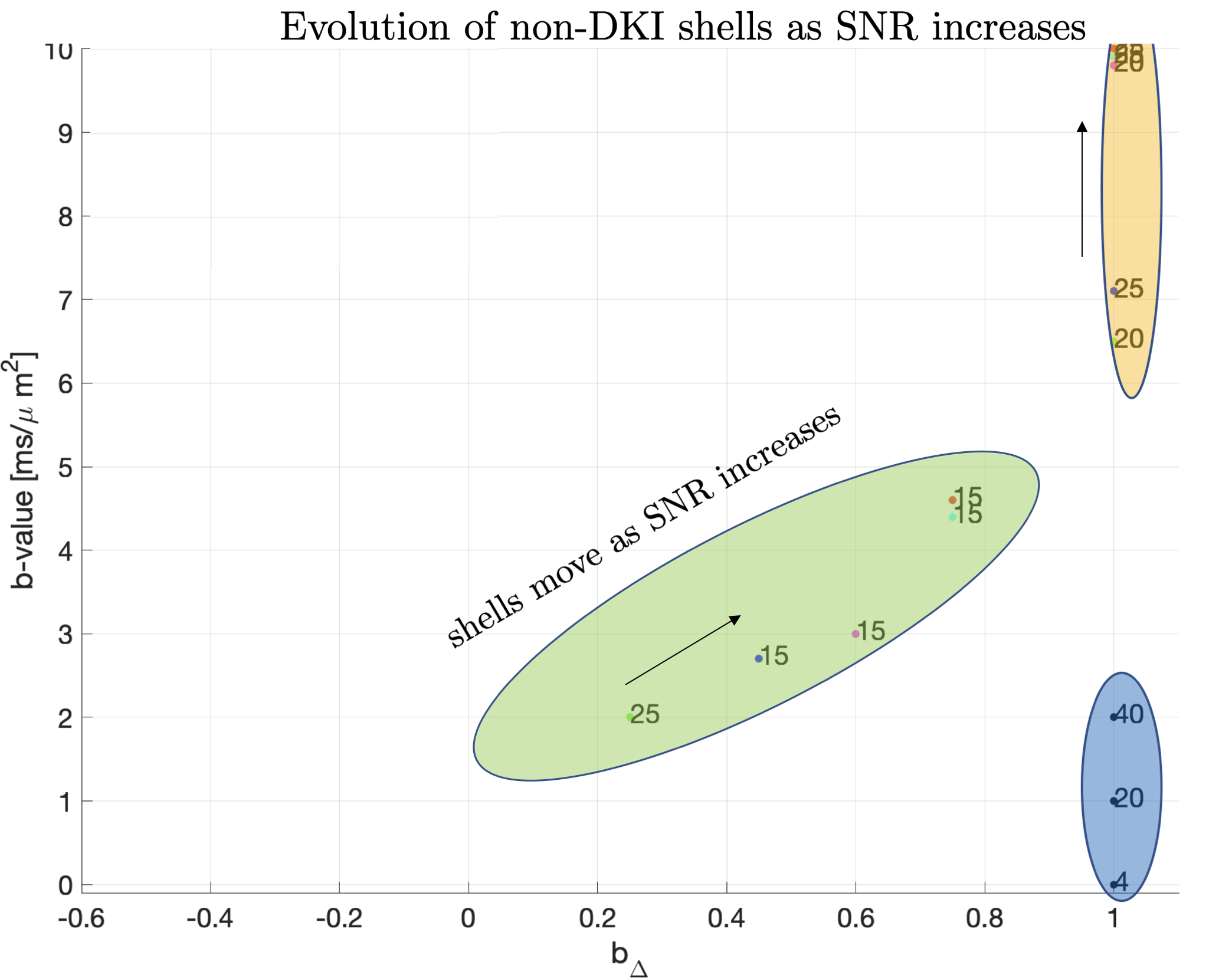
Parameter estimation and protocol optimization metric. For optimal precision we estimate SM parameters using a supervised machine learning method based on polynomial regression from the rotational invariants10. To choose measurements that benefit such estimation the most, we derived an analytical expression for such regression and used it to compute the mean square error (MSE) for a noise propagation experiment with a given protocol and SNR. This has three advantages: first, it is fast to compute, enabling its use as an optimization metric. Second, it accurately captures how our estimates are influenced by trade-offs that are part of the acquisition constraints, e.g. 'more shorter measurements' or 'less longer measurements', see Fig.1. Finally, it provides an accurate estimation of how much SNR impacts results when estimating a broad range of ground truth values. Related work has tackled this problem using Cramer-Rao-bounds on the $$$\mathcal{O}(b^2)$$$ cumulant expansion11 or the SM with diffusion and relaxometry12.Optimisation. Shells of uniformly distributed directions13 were assumed to be part of the optimal acquisition protocol, since it has been shown that measurements grouped into shells increase precision11. Thus, the optimization selected for each shell depends on the diffusion weighting, gradient shape, and number of directions. The echo time (TE) was the same for all shells and determined by the longest diffusion waveform, whereby the optimization selects the optimal shells that minimize our MSE metric The maximum b-values were set to $$$b_{\text{max}}=10ms/\mu m^2$$$ and $$$b_{\text{max}}=8 ms/\mu m^2$$$ to accommodate our two scanners described below. Stochastic optimisation14 was used due to the non-convex optimization landscape. Figure 1 shows how the optimal diffusion protocols vary depending on the signal-to-noise ratio (SNR) considering acquisition settings as described next.
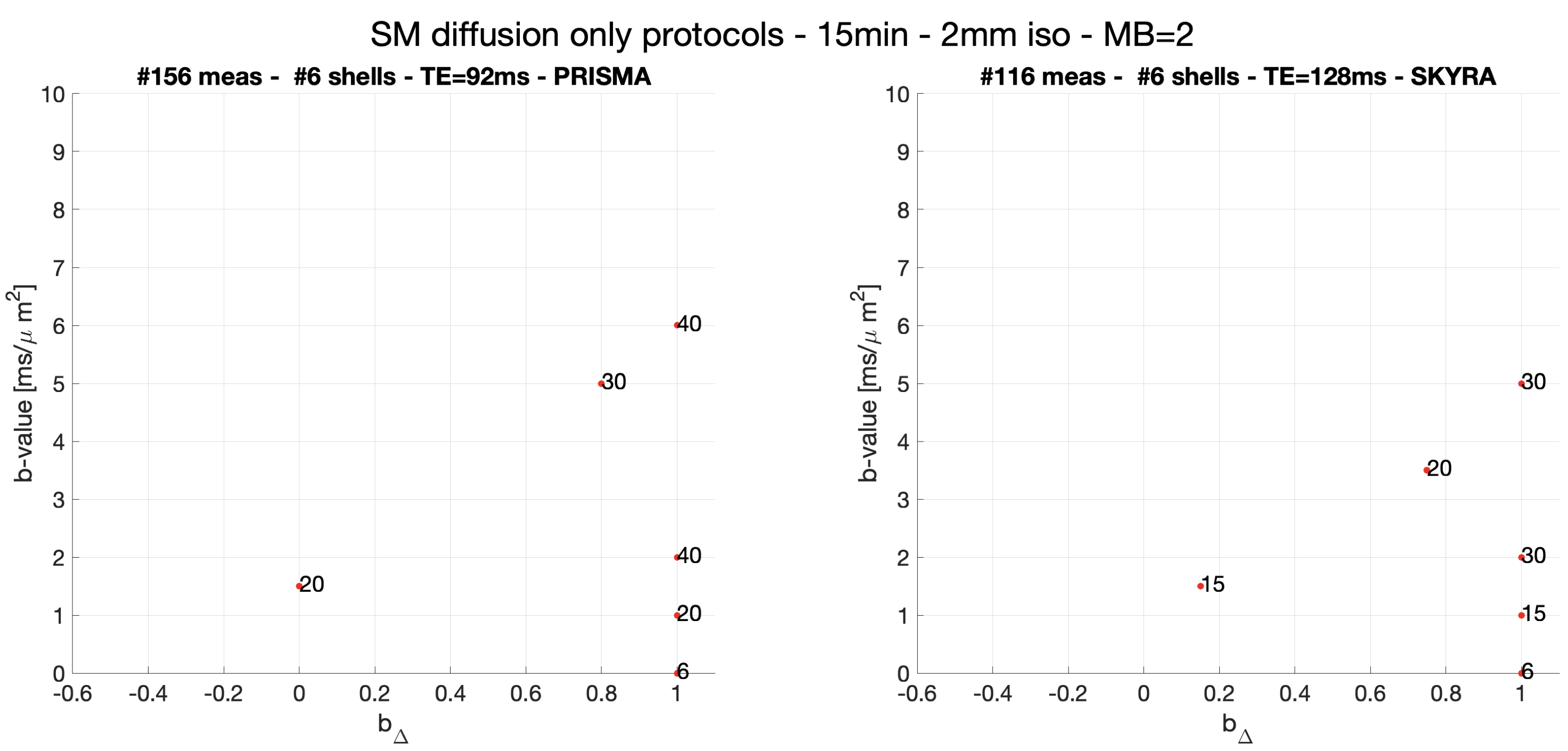
Imaging. After informed consent, three healthy volunteers (female-23yo,male-32yo,male-51yo) underwent brain diffusion (d)MRI on Siemens Magnetom Prisma and Skyra 3T systems ($$$80mT/m$$$ and $$$40mT/m$$$ gradient systems, respectively), using a 20-channel head coil. Maxwell-compensated asymmetric waveforms15 were used in both protocols. Isotropically distributed directions were used at different diffusion weightings (see Fig. 2 for details). On the Skyra scanner, scan(1)-rescan(2) of this protocol was acquired with TR/TE=6700/128ms, while on the Prisma scanner, scan(1)-rescan(2) was acquired with TR/TE=5300/92ms in addition to one scan(3) with TR/TE=6700/128ms. Imaging parameters: resolution: $$$2.0mm$$$ isotropic, in-plane FOV: 220mm, GRAPPA acceleration factor 2, $$$PF=6/8$$$. Data was processed using DESIGNER16,17. Each scan included a reverse phase encoding b=0 image to correct for EPI-induced distortions. Subjects were repositioned between scans.
Results
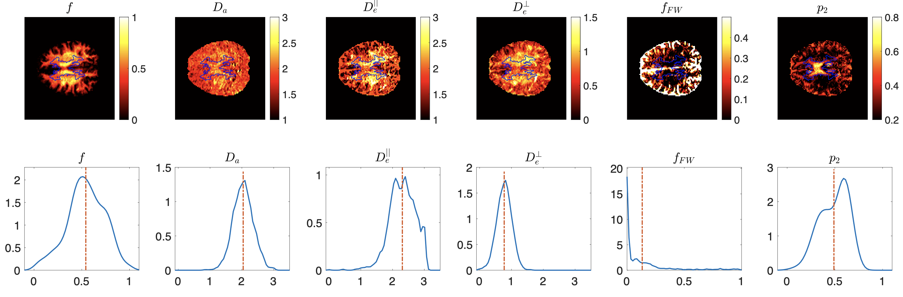
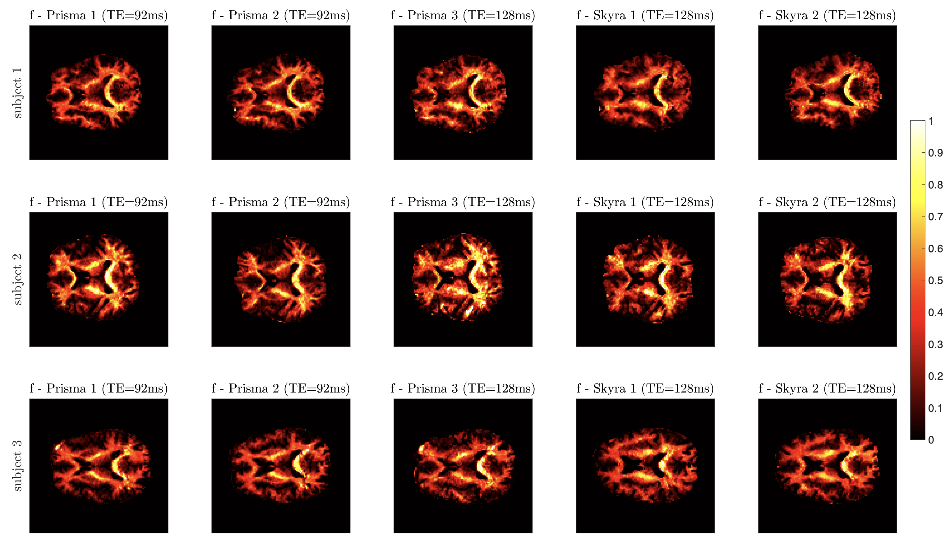
Protocols obtained after optimization for Skyra and Prisma scanners are shown in Fig. 2. Representative WM parametric maps for a 23yo female are shown in Fig. 3, along with corresponding histograms over a WM region of interest. To assess scan-rescan variability, each subject was scanned repeatably on two scanners resulting in 5 scans. Parametric maps of f from each repetition at each scanner are shown in Fig. 4. The coefficients of variation (COV) of the mean estimates for multiple WM ROIs are shown in Fig 5. Remarkably, COV were similar accross scanners and TEs.It was lowest for f, and below 5% for $$$D_a,\,D_e^{||}$$$, while highest for $$$f_{FW}$$$ due to misregistration of the atlas ROIs and the sharp transition between WM and CSF.Discussion and Conclusion
We propose two optimal protocols that maximize accuracy and precision for supervised machine learning parameter estimation, while accounting for hardware limitations related to scanner type (Prisma, Skyra) within 15 minutes scan time. These protocols yield estimates for SM parameters that are in good agreement with reported values using other multidimensional protocols12,18. Using optimized protocols, three healthy volunteers were scanned on different scanners and scan-rescan variability was assessed, yielding good reproducibility-values well within 8%. Due to the combination of denoising, optimal protocols and robust parameter estimation, our method enables estimating standard model parameters in vivo in whole brain white matter in 15 minutes, thereby enabling microstructure mapping in clinical settings. Future work will add relaxometry.Acknowledgements
This work was performed under the rubric of the Center for Advanced Imaging Innovation and Research (CAI2R, https://www.cai2r.net), a NIBIB Biomedical Technology Resource Center (NIH P41-EB017183). This work has been supported by NIH under NINDS award R01 NS088040 and NIBIB awards R01 EB027075.References
[1] D. S. Novikov, E. Fieremans, S. N. Jespersen, and V. G. Kiselev, “Quantifying brain microstructure with diffusion MRI: Theory and parameter estimation,”NMR in Biomedicine, p. e3998, 2018.
[2] I. O. Jelescu, J. Veraart, V. Adisetiyo, S. S. Milla, D. S. Novikov, and E. Fieremans, “One diffusion acquisition and different white matter models: How does microstructure change in human early development based on WMTI and NODDI,”NeuroImage, vol. 107, pp. 242–256, 2015.
[3] I. O. Jelescu, J. Veraart, E. Fieremans, and D. S. Novikov, “Degeneracy in model parameter estimation formulticompartmental diffusion in neuronal tissue,”NMR in Biomedicine, vol. 29, pp. 33–47, 2016.
[4] D. S. Novikov, J. Veraart, I. O. Jelescu, and E. Fieremans, “Rotationally-invariant mapping of scalar and orientational metrics of neuronal microstructure with diffusion MRI,”NeuroImage, vol. 174, pp. 518 – 538, 2018.
[5] S. Coelho, J. M. Pozo, S. N. Jespersen, D. K. Jones, and A. F. Frangi, “Resolving degeneracy in diffusion MRI biophysical model parameter estimation using double diffusion encoding,”Magnetic Resonance in Medicine,vol. 82, pp. 395–410, 2019.
[6] M. Reisert, V. G. Kiselev, and B. Dhital, “A unique analytical solution of the white matter standard model usinglinear and planar encodings,”Magnetic Resonance in Medicine, vol. 81, pp. 3819–3825, 2019.
[7] C.-F. Westin, H. Knutsson, O. Pasternak, F. Szczepankiewicz, E. ̈Ozarslan, D. van Westen, C. Mattisson, M. Bo-gren, L. J. O’Donnell, M. Kubicki, D. Topgaard, and M. Nilsson, “q-space trajectory imaging for multidimensional diffusion MRI of the human brain,”NeuroImage, vol. 135, pp. 345–362, 2016.
[8] D. Topgaard, “Multidimensional diffusion mri,”Journal of Magnetic Resonance, vol. 275, pp. 98–113, 2017.
[9] S. N. Jespersen, C. D. Kroenke, L. Østergaard, J. J. H. Ackerman, and D. A. Yablonskiy, “Modeling dendrite density from magnetic resonance diffusion measurements,”NeuroImage, vol. 34, pp. 1473–1486, 2007.
[10] M. Reisert, E. Kellner, B. Dhital, J. Hennig, and V. G. Kiselev, “Disentangling micro from mesostructure bydiffusion MRI: A Bayesian approach,”NeuroImage, vol. 147, pp. 964 – 975, 2017.
[11] S. Coelho, J. M. Pozo, S. N. Jespersen, and A. F. Frangi, “Optimal experimental design for biophysical modellingin multidimensional diffusion MRI,” in Medical Image Computing and Computer-Assisted Intervention(MICCAI),vol. 3542, Springer, 2019.
[12] Lampinen, B., Szczepankiewicz, F., Mårtensson, J., van Westen, D., Hansson, O., Westin, C.‐F., & Nilsson, M. (2020). Towards unconstrained compartment modeling in white matter using diffusion‐relaxation MRI with tensor‐valued diffusion encoding. Magnetic Resonance in Medicine, 84(3), 1605– 1623.
[13] C. G. Koay, “A simple scheme for generating nearly uniform distribution of antipodally symmetric points on theunit sphere,”Journal of Computational Science, vol. 2, no. 4, pp. 377 – 381, 2011.
[14] I. Zelinka, “Soma — self-organizing migrating algorithm,” in New Optimization Techniques in Engineering, ch. 7,pp. 167–217, Springer Berlin Heidelberg, 2004.
[15] F. Szczepankiewicz, C.-F. Westin, and M. Nilsson, “Maxwell-compensated design of asymmetric gradient wave-forms for tensor-valued diffusion encoding,”Magnetic Resonance in Medicine, vol. 0, pp. 1–14, 2019.
[16] B. Ades-Aron, J. Veraart, P. Kochunov, S. McGuire, P. Sherman, E. Kellner, D. S. Novikov, and E. Fieremans,“Evaluation of the accuracy and precision of the diffusion parameter estimation with gibbs and noise removal pipeline,”NeuroImage, vol. 183, pp. 532 – 543, 2018.
[17] G. Lemberskiy et al. “Mri below the noise floor,” In Proceedings 28nd Scientific Meeting 0770, International Society or Magnetic Resonance in Medicine, Melbourne, Australia, 2020 (2020).
[18] B. Dhital, M. Reisert, E. Kellner, and V. G. Kiselev, “Diffusion weighting with linear and planar encodingsolves degeneracy in parameter estimation,” in Proceedings of the International Society of Magnetic Resonance in Medicine, Wiley, 2018.
[19] D. S. Novikov, V. G. Kiselev, and S. N. Jespersen, “On modeling,”Magnetic Resonance in Medicine, vol. 79,pp. 3172 – 3193, 2018.
Figures
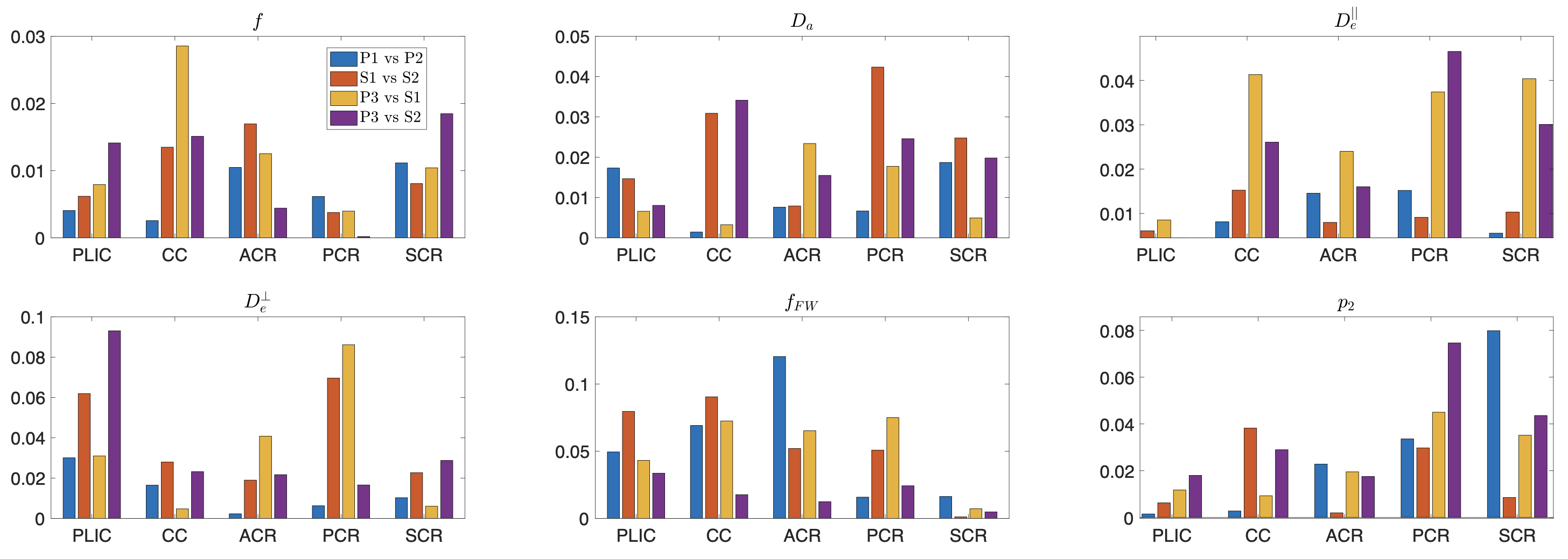
Coefficients of variation (COV$$$=\sigma/\mu$$$) for different ROIs and different scanners (in $$$\mu m^2/ms$$$ for diffusivities). These were averaged over the three subjects and compare pairs of the five acquired datasets, where Prisma 1 (P1) vs. Prisma 2
(P2) and Skyra 1 (S1) vs. Skyra 2 (S2) measure scan-rescan variation
(same scanner, same TE), Prisma 3 (P3) vs. Skyra 1,2 (S) measures
inter-scan variation (varying scanner, fixed TE), and Prisma 1,2 (P) vs
Prisma 3 (P3) measure inter-protocol variation (same scanner, varying
TE). f presents the lowest coefficients of variation.