3408
Impact of within-voxel heterogeneity in fibre geometry on spherical deconvolution
Ross Callaghan1, Daniel C Alexander1, Marco Palombo1, and Hui Zhang1
1Department of Computer Science and Centre for Medical Image Computing, University College London, London, United Kingdom
1Department of Computer Science and Centre for Medical Image Computing, University College London, London, United Kingdom
Synopsis
Axons in white matter have been shown to have varying geometries within a bundle, but what does this mean for spherical deconvolution, which assumes a single diffusion MRI (dMRI) fibre response function (FRF) for all axons within a voxel? We demonstrate, using advanced dMRI simulations, that variable fibre geometry leads to a variable FRF across axons and that a different choice of FRF can lead to large differences in the recovered fibre orientation distribution function (fODF). This finding suggests that assuming a single FRF can lead to misestimation of the fODF, causing further downstream errors in techniques such as tractography.
Introduction
This work investigates how differences in fibre geometries within a voxel impact on spherical deconvolution (SD). SD is a family of techniques that estimates the fibre orientation distribution function (fODF) using diffusion weighted magnetic resonance imaging (dMRI). The approach works by modelling the dMRI signal as a spherical convolution between the fODF and the fibre response function (FRF), the typical signal of a fibre population with a single orientation. By estimating an FRF from voxels where the signals are deemed typical of a single coherent fibre population, the fODF is determined by deconvolving this FRF from the signal1,2. Implicit in this formulation is an assumption that one common FRF is shared across all fibre populations within a voxel. Recent observations from ex-vivo electron microscopy (EM) studies challenge this assumption, showing varying fibre geometries even within a single bundle3–5. This may cause FRF variation across fibres, leading to misestimation of the fODF, which has downstream consequences for techniques including tractography. Here, we investigate the effect of variable fibre geometry using dMRI simulations within realistic digital tissues generated using ConFiG6 and real digital tissues reconstructed from EM3 to demonstrate that fibres within a voxel may not all share the same response. We further evaluate the effect this has on fODF estimates by calculating them using FRFs representing the variable responses present in a voxel.Experiments
1. Variable FRF within voxelWe test to what extent variable fibre geometry results in variable fibre responses by simulating the intracellular dMRI signal from fibres in a range of digital phantoms representing four examples of white matter tissue:
- A single bundle of fibres generated by ConFiG
- Two perpendicular bundles of fibres generated by ConFiG
- Three perpendicular bundles of fibres generated by ConFiG
- Real fibres from mouse corpus callosum reconstructed from EM3
Measurement parameters were ∆=28ms, δ=24ms, b=0,1000,2000,3000s/mm2 and 256 gradient directions per-shell, giving a diffusion time dt=20ms and G=60mT/m at b=3000s/mm2, chosen as a feasible gradient strength on a high-end clinical system. Rician noise was added at 30 SNR.
To demonstrate the variability in dMRI response, each fibre’s response was calculated and the median, 10th and 90th percentile responses found (in terms of mean squared difference between fibre and cylinder responses). Additionally, to relate the type and size of morphological variation to the signal changes, the microscopic orientation dispersion7 ($$$\mu OD$$$), a measure of undulation, and the coefficient of variation of diameter ($$$CV$$$), a measure of beading8, was calculated for each fibre.
2. Impact on fODF estimation
To investigate the impact on the fODF of assuming a single fibre response per voxel, we compared fODF estimates from constrained spherical deconvolution (CSD)9 using three different FRFs per phantom: the median response from Experiment 1 (representing a typical response) and the 10th percentile and 90th percentile FRF (representing extrema of responses). A gold standard fODF was generated by projecting the end points of each fibre onto a triangulated sphere as in 3,6. To quantify differences in the fODFs, the main peak direction and dispersion angle (angle away from main direction to cover 75th percentile of main peak) were calculated for the single bundle and EM fibre cases.
Results and Discussion
Variable FRF within voxelVariations in intra-voxel fibre geometries are present in real fibres and ConFiG phantoms as demonstrated in Figure 2 which shows each digital phantom alongside the fibres which give the median, 10th and 90th percentile response. Under the experimental conditions investigated, this variability in fibre geometry leads to variable FRFs. Phantoms which show large amounts of beading (high $$$CV$$$ in EM fibres and three crossing bundles) show the largest variability in response, while $$$\mu OD$$$ affects the response less, suggesting that fibre beading drives fibre response variability more than undulation.
Impact on fODF estimation
The FRF used in CSD can have a large impact on the resulting fODF even when the difference in FRF is relatively small as demonstrated by Figures 3&4. There is generally no single choice of FRF that works best for all scenarios, with median working well for EM fibres, but 10th percentile best for One Bundle. For crossing bundles, fODF directions are well estimated, though peak amplitudes change with different FRFs.
Conclusion
We have demonstrated that intra-voxel heterogeneity in fibre geometry leads to variable dMRI responses per-fibre, with fibre beading playing an important role. This variability means that the assumption of any single FRF for all fibres in a voxel may lead to a poor estimation of the fODF, including peak direction and relative amplitude errors, which could have large consequences for subsequent methods using the fODF such as tractography. This study only considers intra-axonal signal, however while future work will investigate the impact of realistic extra-axonal space on SD, these results should hold for high b-values.Acknowledgements
This work is supported by the EPSRC-funded UCL Centre for Doctoral Training in Medical Imaging (EP/L016478/1) and the Department of Health’s NIHR-funded Biomedical Research Centre at University College London Hospitals. This work was supported by EPSRC grants EP/M020533/1 and EP/N018702/1. MP is supported by UKRI Future Leaders Fellowship (MR/T020296/1)References
- Tournier JD, Calamante F, Gadian DG, Connelly A. Direct estimation of the fiber orientation density function from diffusion-weighted MRI data using spherical deconvolution. NeuroImage. 2004;23(3):1176-1185. doi:10.1016/j.neuroimage.2004.07.037
- Dell’Acqua F, Tournier JD. Modelling white matter with spherical deconvolution: How and why? NMR in Biomedicine. 2019;32(4):1-18. doi:10.1002/nbm.3945
- Lee HH, Yaros K, Veraart J, et al. Along-axon diameter variation and axonal orientation dispersion revealed with 3D electron microscopy : implications for quantifying brain white matter microstructure with histology and diffusion MRI. Brain Structure and Function. 2019;224:1469-1488. doi:10.1007/s00429-019-01844-6
- Abdollahzadeh A, Ilya B, Jokitalo E, Tohka J, Sierra A. Automated 3D Axonal Morphometry of White Matter. Scientific Reports. 2019;9:1-16. doi:10.1038/s41598-019-42648-2
- Salo RA, Belevich I, Jokitalo E, Gröhn O, Sierra A. Assessment of the structural complexity of diffusion MRI voxels using 3D electron microscopy in the rat brain. NeuroImage. 2021;225:117529. doi:10.1016/j.neuroimage.2020.117529
- Callaghan R, Alexander DC, Palombo M, Zhang H. ConFiG: Contextual Fibre Growth to generate realistic axonal packing for diffusion MRI simulation. NeuroImage. 2020;220:117107. doi:10.1016/j.neuroimage.2020.117107
- Brabec J, Lasič S, Nilsson M. Time-dependent diffusion in undulating thin fibers: Impact on axon diameter estimation. NMR in Biomedicine. 2019;(February 2019):1-19. doi:10.1002/nbm.4187
- Lee H, Papaioannou A, Kim S-L, Novikov DS, Fieremans E. A time-dependent diffusion MRI signature of axon caliber variations and beading. Communications Biology. 2020;(2020). doi:10.1038/s42003-020-1050-x
- Tournier JD, Calamante F, Connelly A. Robust determination of the fibre orientation distribution in diffusion MRI: Non-negativity constrained super-resolved spherical deconvolution. NeuroImage. 2007;35(4):1459-1472. doi:10.1016/j.neuroimage.2007.02.016
Figures
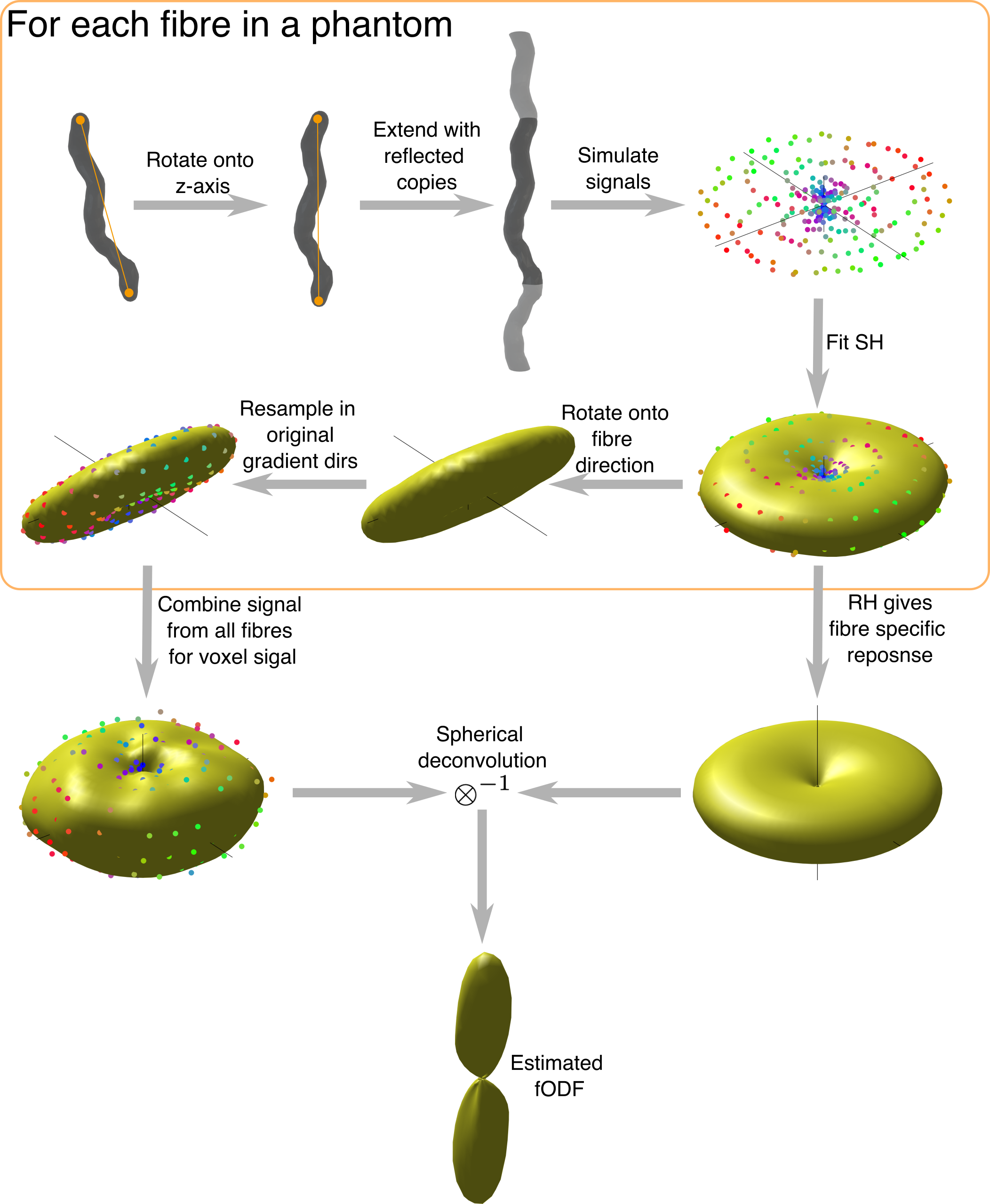
Figure 1. Method for simulating FRFs and estimating fODFs. Each fibre is aligned with the z-axis and extended with reflected copies to avoid simulation artefacts from closed fibres. Simulated signal is generated only from spins within the original fibre copy. The spherical harmonic decomposition of each fibre is found and the rotational harmonics give the FRF. To generate overall voxel signal, the SH signal is rotated onto the original fibre direction and combined from each fibre, weighted by fibre volume. This signal is then deconvolved with the desired FRF to estimate the fODF.
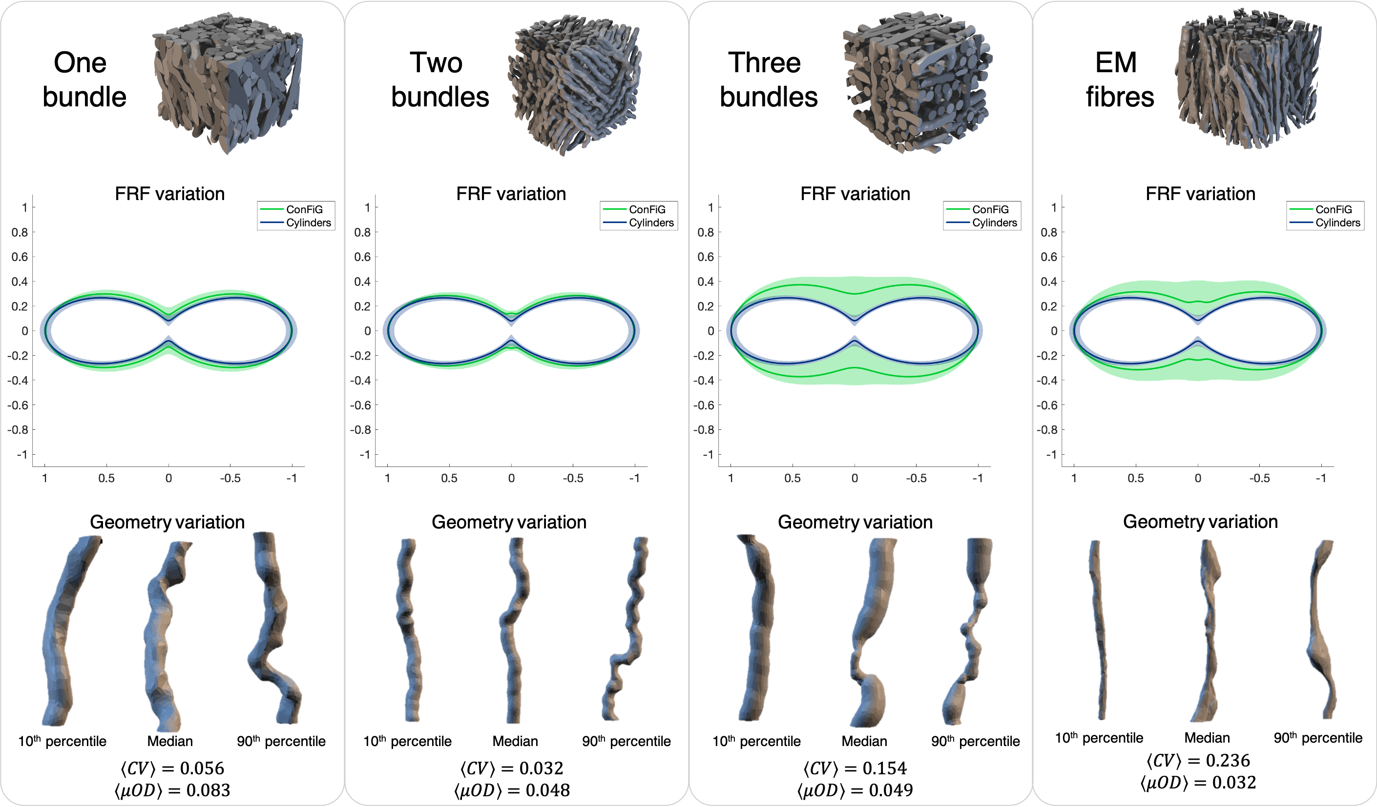
Figure 2. Variability in fibre responses within a voxel at b=2000 s/mm2 along with geometrical variation in fibres responsible for median, 10th and 90th percentile response. Notably, the 10th percentile fibres tend to be more stick-like while 90th percentile have more beading. Solid green line in FRF figures represents median response, shaded green area represents 10th and 90th percentile response. Same values for representative cylinders are in blue to demonstrate the variability due to noise.
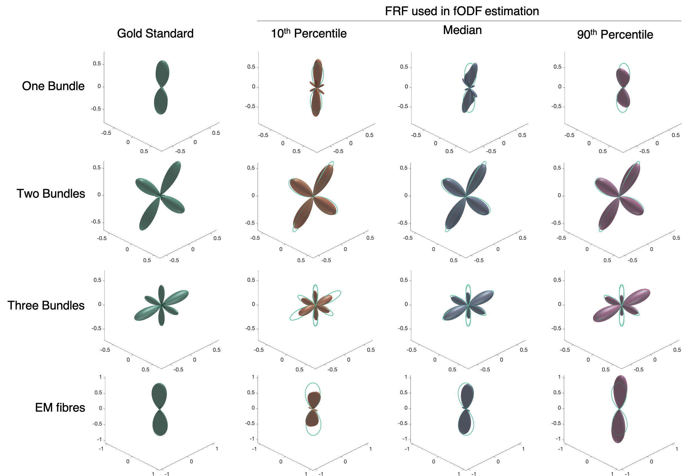
Figure 3. fODFs estimated using different FRFs showing how assuming a different FRF can result in vastly different fODFs. Green outline in rightmost plots shows gold standard fODF for comparison. All fODFs are normalised to integrate to 1 for comparison.
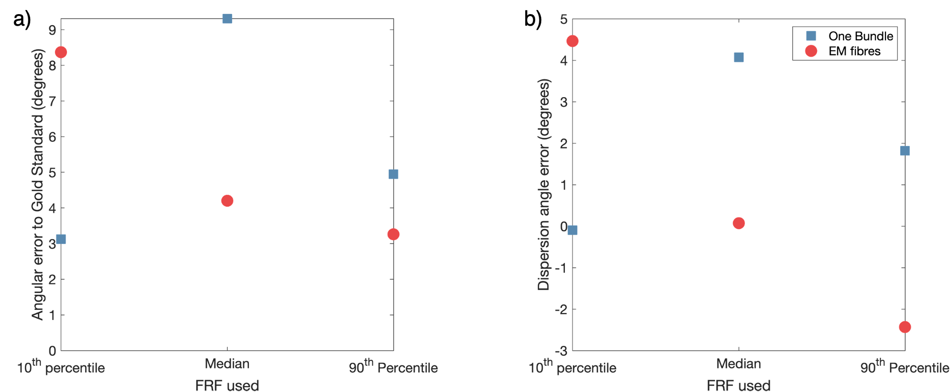
Figure 4. Variation in fODF properties when estimated using different FRFs. a) the angular error between the main peak in gold standard fODF and that of the fODFs estimated using CSD and b) the error in dispersion angle of the main peak (angle from main peak direction to cover 75th percentile) compared to the gold standard for each fODF