3400
Simulating the BOLD fMRI transverse relaxation at 3 T: How accurate is the 2D approximation?1Rotman Research Institute, Baycrest Health Sciences, North York, ON, Canada, 2A. A. Martinos Center for Biomedical Imaging, Harvard Medical School, Massachusetts General Hospital, Boston, MA, United States, 3Department of Medical Biophysics, University of Toronto, Toronto, ON, Canada
Synopsis
Biophysical simulations of the BOLD fMRI phenomenon are indispensable for the development of quantitative fMRI techniques. Since the “gold-standard” 3D Monte Carlo simulation approach was proposed, 2D variations that are less computationally intensive have also been suggested. However, these approaches have never been directly compared. In this work, we directly compare the accuracy of 2D approaches against 3D ones, in order to reconcile results from different simulation studies.
Introduction
Simulating the biophysics of BOLD contract is indispensable to expand the utility of BOLD fMRI towards quantitative measurements of brain metabolism and hemodynamics 1–3. Since the initial work by Ogawa et al. 4, 3D Monte Carlo (MC) simulations of transverse relaxation have been regarded as the de facto gold-standard approach 5–7. Nonetheless, this approach is rather resource intensive in terms of computer memory and speed 8. To combat this, Bandettini and Wong proposed the deterministic diffusion method in 2D, which significantly reduces computational requirements and accelerates BOLD simulations 9. 2D techniques have since been applied for both deterministic diffusion and MC simulations. However, despite a consistent stream of studies using either 2D or 3D simulations, results from the two have not been systematically compared with one another with the same assumed parameters, potentially impeding the reconciliation of results from different studies. Here, we compare MC simulations of BOLD relaxation using 2D and 3D vessel networks.Methods
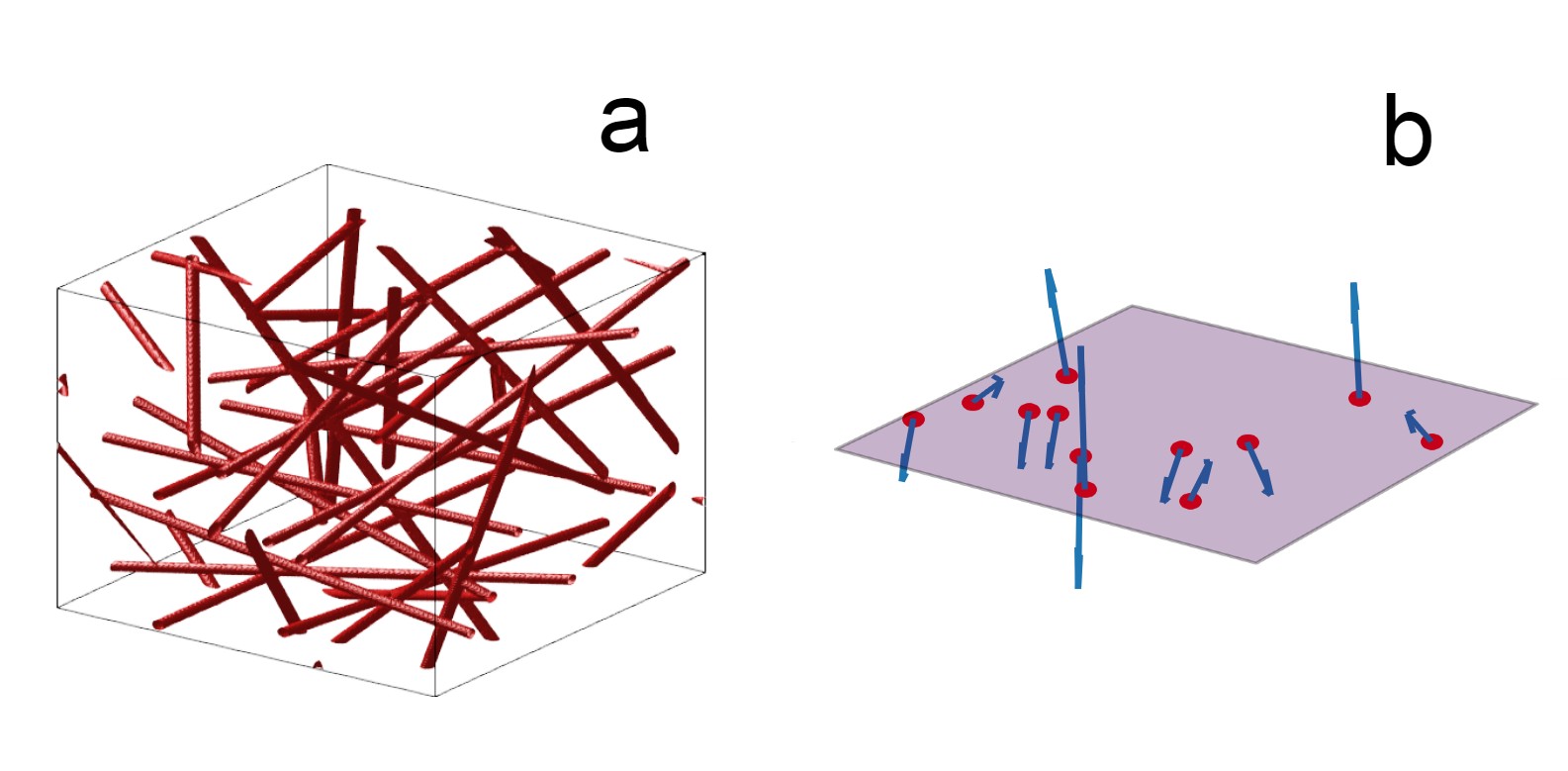
Voxel generation: The 2D and 3D models differ significantly. All approaches are implemented as custom scripts in Python.For 3D, a spherical space is filled with 300 randomly oriented and positioned infinite cylindrical vessels. To ensure uniform volume density distribution, these parameters are calculated as described by Martindale et al. 8. The vessel volume is approximated analytically and iteratively adds to the cerebral blood volume (CBV) until it is reached. Figure 1-a shows a simplified version of a generated 3D voxel. For 2D, a square plane is created with 300 perturbers as well. All vessel axes are oriented orthogonally to the plane, generating circular cross sections 1. Randomization of vessel orientations is implemented as a uniform distribution of random B0 directions, as proposed by Miller et al. 10. This ensured that CBV is simply the sum of all vessel cross-sections on the plane. Figure 1-b represents the implementation of the voxel plane in the 2D simulation. When comparing the two methods, CBV was matched. The 3D and 2D off-resonance (Δω) maps are then calculated analytically with the equations from Ogawa et al. 4, assuming a B0 of 3 T.
Diffusion process: Extravascular Monte Carlo spin diffusion is implemented in both the 2D and 3D methods using 5000 spins, randomly positioned outside the vessels. These spins are allowed to diffuse in the extravascular space using Einstein’s method at a diffusion coefficient of 1μm2/ms. The position of all spins are tracked in physical units as they accumulate phase through diffusion. This method is prefered to the alternative creation of a discretized phase accumulation grid as it is quasi-infinitely accurate and is faster in the case of short time spans. The time step used was 0.2 ms.
R2’ calculation: The signal is calculated as the mean dephasing of all spins at each dt, but also depends on the pulse sequence. The reversible transverse relaxation (R2’) is calculated from this signal at the echo time (TE) using the exponential decay model. We do so for gradient-echo (GE), spin-echo (SE) and asymmetric spin-echo (ASE) contrast. The target TEs are 30ms for GE, 70ms for SE and 70ms for ASE. For ASE, the time shift τ is 50ms.
Results
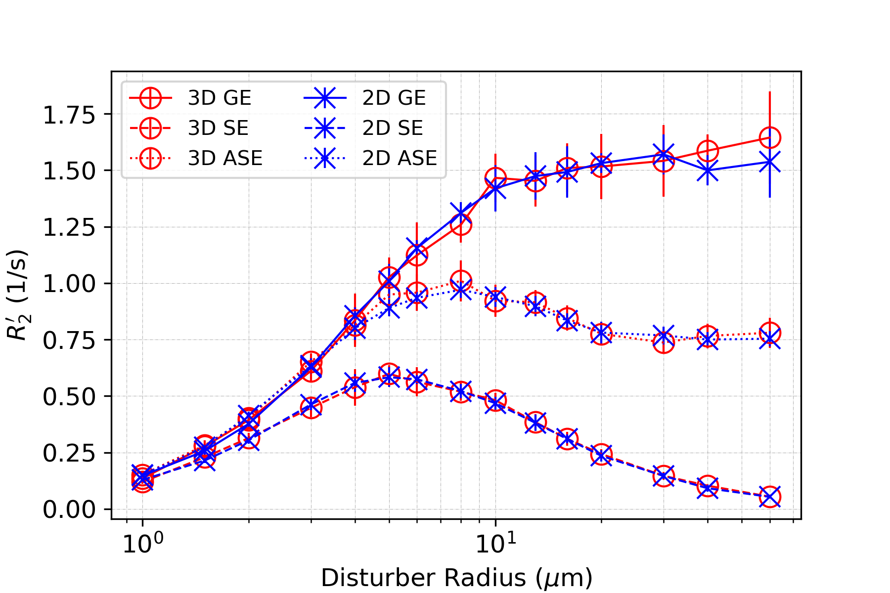
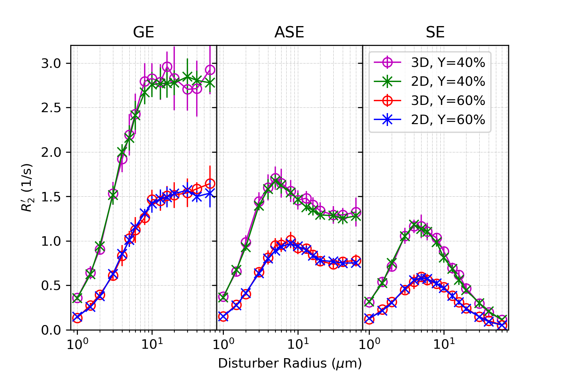
In all figures, data points are the mean of simulation across 10 iterations of vessel networks with the standard deviation shown by error bars. In Figure 2, we show the R2’ vs. vessel radius plots for all pulse sequences, demonstrating excellent agreement between 2D and 3D methods for all three pulse sequences. The curves also match the expected behaviour observed by Boxerman et al. 5; the GE curve experiences a plateau at large diameters while the SE and ASE sequences exhibit an R2’ peak, the ASE peak being at a slightly larger diameter.As shown in Figure 3 and 4, the excellent agreement between 2D and 3D methods is also maintained when observing the R2’ vs. CBV and R2’ vs. oxygenation (Y) relationships. The R2’ values (Figure 3) conform to the linear relationship expected from Boxerman’s work 5 and are consistent across the simulation methods. Figure 4 shows the diameter dependence of R2’ for the pulse sequences at two different blood oxygenations, 40% and 60%. Increasing the susceptibility difference between blood and tissue (equivalent to decreasing Y) causes R2’ to increase and its peak to shift to a smaller diameter, also in agreement with Boxerman et al. 5.
Discussion
In this work, we show that the 2D voxel approximation produces BOLD simulation results that are practically identical to those of the “gold-standard” 3D voxel approach. This finding establishes the validity of the 2D approximation as a faster, less memory-intensive alternative, which is appropriate when complete vascular anatomical realism is not required 11,12. While the presented results are based on MC diffusion, our comparison of 3D MC vs. 2D deterministic diffusion simulations is also underway, as well as the incorporation of intravascular effects.Acknowledgements
We thank the Canadian Institutes for Health Research (CIHR) (grant MFE-164755 and grant FRN# 148398) and the Natural Sciences and Engineering Research Council of Canada (NSERC) (grant FGPIN# 418443) for financial support.References
1. Berman, A. J. L. et al. Gas-free calibrated fMRI with a correction for vessel-size sensitivity. Neuroimage 169, 176–188 (2018).
2. Blockley, N. P., Griffeth, V. E. M., Simon, A. B., Dubowitz, D. J. & Buxton, R. B. Calibrating the BOLD response without administering gases: comparison of hypercapnia calibration with calibration using an asymmetric spin echo. Neuroimage 104, 423–429 (2015).
3. Christen, T. et al. MR vascular fingerprinting: A new approach to compute cerebral blood volume, mean vessel radius, and oxygenation maps in the human brain. Neuroimage 89, 262–270 (2014).
4. Ogawa, S. et al. Functional brain mapping by blood oxygenation level-dependent contrast magnetic resonance imaging. A comparison of signal characteristics with a biophysical model. Biophysical Journal vol. 64 803–812 (1993).
5. Boxerman, J. L., Hamberg, L. M., Rosen, B. R. & Weisskoff, R. M. MR contrast due to intravascular magnetic susceptibility perturbations. Magn. Reson. Med. 34, 555–566 (1995).
6. Weisskoff, R. M., Zuo, C. S., Boxerman, J. L. & Rosen, B. R. Microscopic susceptibility variation and transverse relaxation: theory and experiment. 31, 601–610 (1994).
7. Báez-Yánez, M. G. et al. The impact of vessel size, orientation and intravascular contribution on the neurovascular fingerprint of BOLD bSSFP fMRI. Neuroimage 163, 13–23 (2017).
8. Martindale, J., Kennerley, A. J., Johnston, D., Zheng, Y. & Mayhew, J. E. Theory and generalization of Monte Carlo models of the BOLD signal source. Magn. Reson. Med. 59, 607–618 (2008).
9. Bandettini, P. A. & Wong, E. C. Effects of biophysical and physiologic parameters on brain activation-induced R2* and R2 changes: simulations using a deterministic diffusion model. Int. J. Imaging Syst. Technol. 6, 133–152 (1995).
10. Miller KL, Jezzard P. Modeling SSFP functional MRI contrast in the brain. Magn Reson Med 2008;60:661–673 doi: 10.1002/mrm.21690.
11. Gagnon L, Sakadžić S, Lesage F, et al. Quantifying the microvascular origin of bold-fMRI from first principles with two-photon microscopy and an oxygen-sensitive nanoprobe. J. Neurosci. 2015;35:3663–3675 doi: 10.1523/JNEUROSCI.3555-14.2015.
12. Baez-Yanez MG, Ehses P, Mirkes C, Tsai PS, Kleinfeld D, Scheffler K. The impact of vessel size, orientation and intravascular contribution on the neurovascular fingerprint of BOLD bSSFP fMRI. Neuroimage 2017;163:13–23 doi: 10.1016/j.neuroimage.2017.09.015.
Figures