3398
Biophysical simulations of the BOLD fMRI signal using realistic imaging gradients: Understanding macrovascular contamination in Spin-Echo EPI1Athinoula A. Martinos Center for Biomedical Imaging, Massachusetts General Hospital, Charlestown, MA, United States, 2Department of Radiology, Harvard Medical School, Boston, MA, United States, 3Harvard-MIT Division of Health Sciences and Technology, Massachusetts Institute of Technology, Cambridge, MA, United States, 4Department of Radiology, Stanford University, Palo Alto, CA, United States, 5Department of Electrical Engineering, Stanford University, Palo Alto, CA, United States, 6Rotman Research Institute, Baycrest Health Sciences, Toronto, ON, Canada, 7Department of Medical Biophysics, University of Toronto, Toronto, ON, Canada
Synopsis
We introduce simulations of the BOLD signal that incorporate realistic image encoding gradients to help better understand the role the acquisition window plays on BOLD contrast. We applied this framework to examine the well-known macrovascular R2' contamination in spin-echo EPI BOLD signals as a function of readout duration, vessel diameter, and voxel size using randomly oriented cylinders. To understand large-vessel effects, more realistic anatomy is needed; therefore, we added a large pial vein to random microvascular networks to systematically investigate macrovascular contamination along cortical depths and across columns. This framework reproduced experimentally established results related to the acquisition window duration.
Introduction
Biophysical simulations of the blood-oxygenation-level-dependent (BOLD) signal have provided valuable insights into BOLD contrast mechanisms.1–4 This includes the finding that spin-echo (SE) BOLD has reduced macrovascular sensitivity compared to gradient-echo (GE) BOLD,3 making it potentially more specific to neuronal activation.5,6 Generally, BOLD simulation studies consider the signal at the echo-time (TE) and ignore spatial encoding. Yet, experimentally, fMRI is typically performed with echo-planar imaging (EPI) that samples signal far from the echo. This lengthy readout results in geometric artifacts,7–9 can reduce GE-BOLD sensitivity,10 and can introduce R2' contamination into SE-BOLD, resulting in undesired macrovascular sensitivity.11–13Here, we incorporate realistic image-encoding gradients into BOLD simulations to better understand the role the acquisition window plays on BOLD contrast in practice. We apply this framework to examine macrovascular contamination in SE-BOLD signals as a function of readout duration, vessel diameter, and voxel size using randomly oriented cylinders. Finally, to understand experimentally reported macrovascular contamination data,12,13 we included additional anatomical realism by modelling large pial veins and calculated how their contributions decrease with cortical depth.
Methods
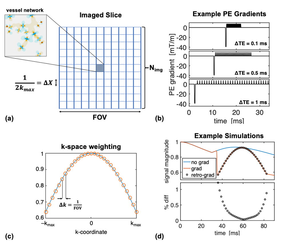
Simulations were performed using the deterministic diffusion method with impermeable vessels.14–16 Figure 1a shows a schematic of the imaging slice, where the simulated voxel is surrounded by zero magnetization. EPI phase-encoding (PE) gradients were modelled using a maximum amplitude of 40 mT/m and the minimum time possible for the prephaser and blips (Figure 1b). PE echo-spacings (ΔTE) were multiples of the simulation time-step, dt. Frequency-encoding was ignored.At each echo of the EPI echo train, the imposed k-space weighting was$$$\;\Delta X\cdot\text{sinc}(k\Delta X)\;$$$and the echoes were combined to form a projection along y using:$$I(y)=\frac{1}{N}\sum_{n=-N/2}^{N/2-1}{S(\text{TE}_n)\cdot\text{sinc}(\Delta X\cdot k_n)\cdot e^{i2\pi k_ny}}.\;\;\;\;\;(1)$$Given that the magnetization is only at $$$y=0$$$, this simplifies to$$I(y=0)=\frac{1}{N}\sum_{n=-N/2}^{N/2-1}{S(\text{TE}_n)\cdot\text{sinc}(\Delta X\cdot k_n)}, \;\;\;\;\;(2)$$which is effectively the average of the sinc-weighted signal. Based on Eq. (2), we also retrospectively scaled simulations without PE gradients by applying the desired k-space weighting at each echo of the echo-train and found comparable results to the simulations with explicit gradients (Figure 1d).
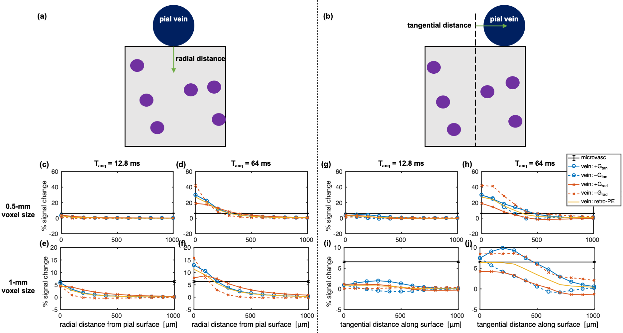
We added to the simulations a large vein, perpendicular to B0, along a “pial surface” atop a random microvascular network of 4-μm radius vessels. Its position was shifted radially and tangentially relative to the sampling region to examine the depth-dependence and tangential distance-dependence of the macrovascular contamination (Figure 4a–b).
Simulations were at 3T and 7T using 64 voxels in the imaging slice with ΔTE = (0, 0.2, 0.5, 1) ms (giving acquisition durations, Tacq, of 0–64 ms), dt=0.1 ms, TE=70 ms. This longer TE was required to achieve the longest Tacq of 64 ms. Vessel networks used cerebral blood volume (CBV)=2%, blood oxygenation (sO2)=60% at baseline and 70% at activation, and hematocrit=40%. Intrinsic T2 of tissue and blood were included using published expressions.4
Results
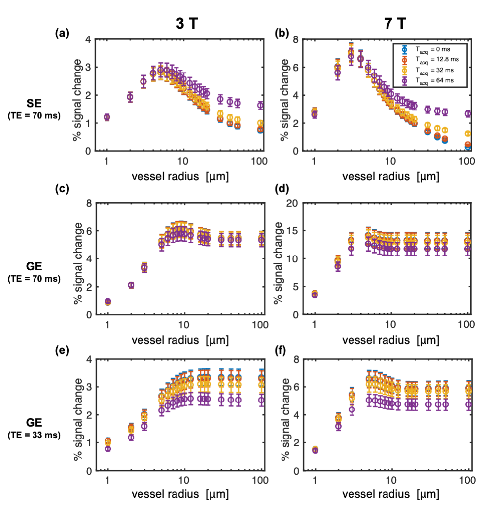
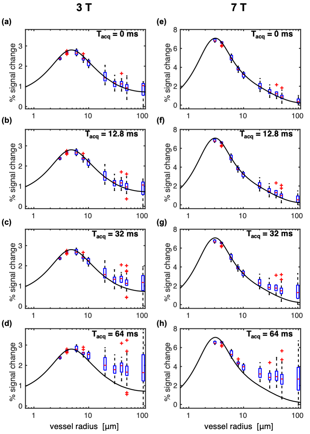
Figure 2 shows the impact of vessel radius and acquisition duration (Tacq) on percent signal change (%S) in simulations where the voxel size was scaled with radius so as to contain a fixed number of vessels, as is conventionally done.3,14–18 Surprisingly, %S increased very little even for the largest radius of 100 μm.The simulations above were repeated with a fixed voxel size of 1.2 mm such that there was only a single vessel constituting the 2% CBV for a 100-μm radius. Figure 3 shows how this generates more variability in %S for the largest radii, including much greater %S values for the longest Tacq, in-line with previous experimental findings.12,13 This has important implications when the voxel has partial voluming with large vessels.
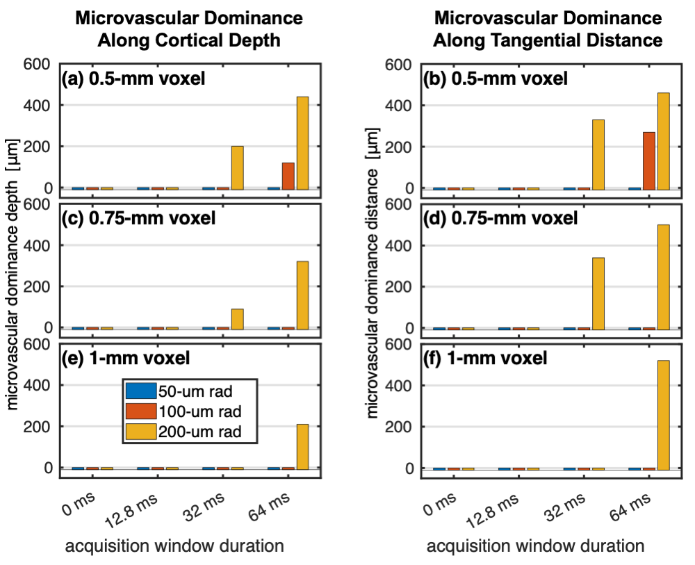
Figure 4 shows the depth- and tangential distance-dependence of the microvascular and pial vein %S. There was a notable effect of the gradient direction and polarity on the pial %S due to the asymmetry of the field from the single vessel. However, the retrospective k-space weighting conveniently captured the approximate average behaviour. Figure 5 shows the distance of microvascular dominance, where the microvascular %S became twice the pial %S.19
Discussion
We have presented a new framework that introduces more realism into biophysical MR simulations by either explicitly or retrospectively incorporating the effects of image-encoding gradients. With this, we reproduced the experimentally observed increase in R2' contamination in SE-EPI-BOLD from large vessels for extended acquisition durations. This was most deleterious when the voxel size was small enough to be impacted by a few large vessels. Direction and polarity of the PE gradient differentially affected macrovascular contamination, suggesting that columnar analyses of SE-EPI-BOLD may show more regionally varying sensitivity, whereas this may average out in laminar analyses. Contamination from large pial vessels did fall off relatively rapidly with distance in the cortex, perhaps suggesting that large-vessel contamination arises mostly from partial volume effects at the pial surface, which appears consistent with Goense and Logothetis.12Most of the simulated %S values were higher than what is typically observed experimentally. This is potentially due to several factors, including using large sO2 changes across all vessels and ignoring CBV changes. To address this, we will test a range of sO2 and CBV changes and apply our framework to more realistic anatomy and physiology.20–22 In future work, we will build on this framework to investigate 3D-GRASE,23 and plan to validate these results using a microsphere phantom.24
Acknowledgements
This work was supported in part by the CIHR (fellowship MFE-164755 and grant FRN# 148398) the NIH NIBIB (grants P41-EB030006, R01-EB019437), by the BRAIN Initiative (NIH NIMH grants R01-MH111419 and R01-MH111438, and NIBIB grant U01-EB025162), NSERC (grant FGPIN# 418443), and by the MGH/HST Athinoula A. Martinos Center for Biomedical Imaging; and was made possible by the resources provided by NIH Shared Instrumentation Grants S10-RR023043 and S10-OD023637.References
1. Ogawa S, Menon RS, Tank DW, et al. Functional brain mapping by blood oxygenation level-dependent contrast magnetic resonance imaging. A comparison of signal characteristics with a biophysical model. Biophys J 1993;64:803–812 doi: 10.1016/S0006-3495(93)81441-3.
2. Weisskoff RM, Zuo CS, Boxerman JL, Rosen BR. Microscopic susceptibility variation and transverse relaxation: theory and experiment. Magn Reson Med 1994;31:601–610.
3. Boxerman JL, Hamberg LM, Rosen BR, Weisskoff RM. MR Contrast Due to Intravascular Magnetic-Susceptibility Perturbations. Magn Reson Med 1995;34:555–566.
4. Uludag K, Muller-Bierl B, Ugurbil K. An integrative model for neuronal activity-induced signal changes for gradient and spin echo functional imaging. Neuroimage 2009;48:150–165 doi: 10.1016/j.neuroimage.2009.05.051.
5. Norris DG. Spin-echo fMRI: The poor relation? Neuroimage 2012;62:1109–1115 doi: 10.1016/j.neuroimage.2012.01.003.
6. Koopmans PJ, Yacoub E. Strategies and prospects for cortical depth dependent T2 and T2* weighted BOLD fMRI studies. Neuroimage 2019;197:668–676 doi: 10.1016/j.neuroimage.2019.03.024.
7. Farzaneh F, Riederer SJ, Pelc NJ. Analysis of T2 limitations and off‐resonance effects on spatial resolution and artifacts in echo‐planar imaging. Magn. Reson. Med. 1990;14:123–139 doi: 10.1002/mrm.1910140112.
8. Haacke EM, Brown RW, Thompson MR, Venkatesan R. Magnetic Resonance Imaging: Physical Principles and Sequence Design. 1st ed. New York: John Wiley & Sons; 1999.
9. Jezzard P, Balaban RS. Correction for geometric distortion in echo planar images from B0 field variations. Magn. Reson. Med. 1995;34:65–73 doi: 10.1002/mrm.1910340111.
10. Buxton RB. Introduction to Functional Magnetic Resonance Imaging: Principles and Techniques. 2nd ed. Cambridge ; New York: Cambridge University Press; 2009.
11. Birn RM, Bandettini PA. The effect of T2’ changes on spin-echo EPI-derived brain activation maps. In: Proceedings of the 10 th Annual Meeting of ISMRM. Vol. 10. ; 2002. p. 1324.
12. Goense JB, Logothetis NK. Laminar specificity in monkey V1 using high-resolution SE-fMRI. Magn Reson Imaging 2006;24:381–392 doi: 10.1016/j.mri.2005.12.032.
13. Wang F, Dong Z, Tian Q, et al. Cortical-depth dependence of pure T2-weighted BOLD fMRI with minimal T2’ contamination using Echo-Planar Time-resolved Imaging (EPTI). Proc Intl Soc Mag Reson Med 2020;28:1229.
14. Bandettini PA, Wong EC. Effects of Biophysical and Physiological-Parameters on Brain Activation-Induced R(2)Asterisk and R(2) Changes - Simulations Using a Deterministic Diffusion-Model. Int. J. Imaging Syst. Technol. 1995;6:133–152 doi: Doi 10.1002/Ima.1850060203.
15. Pannetier NA, Sohlin M, Christen T, Schad L, Schuff N. Numerical modeling of susceptibility-related MR signal dephasing with vessel size measurement: Phantom validation at 3T. Magn Reson Med 2014;72:646–658 doi: 10.1002/mrm.24968.
16. Berman AJL, Mazerolle EL, MacDonald ME, Blockley NP, Luh WM, Pike GB. Gas-free calibrated fMRI with a correction for vessel-size sensitivity. Neuroimage 2018;169:176–188 doi: 10.1016/j.neuroimage.2017.12.047.
17. Martindale J, Kennerley AJ, Johnston D, Zheng Y, Mayhew JE. Theory and generalization of Monte Carlo models of the BOLD signal source. Magn Reson Med 2008;59:607–618 doi: 10.1002/mrm.21512. 18. Dickson JD, Ash TW, Williams GB, et al. Quantitative BOLD: the effect of diffusion. J Magn Reson Imaging 2010;32:953–961 doi: 10.1002/jmri.22151.
19. Pfannmoeller JP, Berman AJL, Kura S, Cheng X, Boas DA, Polimeni JR. Quantification of draining vein dominance across cortical depths in BOLD fMRI from first principles using realistic Vascular Anatomical Networks. In: Proceedings of the 27th Annual Meeting of ISMRM. Montreal, Canada; 2019. p. 3715.
20. Gagnon L, Sakadžić S, Lesage F, et al. Quantifying the microvascular origin of bold-fMRI from first principles with two-photon microscopy and an oxygen-sensitive nanoprobe. J. Neurosci. 2015;35:3663–3675 doi: 10.1523/JNEUROSCI.3555-14.2015.
21. Baez-Yanez MG, Ehses P, Mirkes C, Tsai PS, Kleinfeld D, Scheffler K. The impact of vessel size, orientation and intravascular contribution on the neurovascular fingerprint of BOLD bSSFP fMRI. Neuroimage 2017;163:13–23 doi: 10.1016/j.neuroimage.2017.09.015.
22. Hartung G, Vesel C, Morley R, et al. Simulations of blood as a suspension predicts a depth dependent hematocrit in the circulation throughout the cerebral cortex. PLoS Comput. Biol. 2018;14 doi: 10.1371/journal.pcbi.1006549.
23. Feinberg DA, Harel N, Ramanna S, Ugurbil K, Yacoub E. Sub‐millimeter single‐shot 3D GRASE with inner volume selection for T2 weighted fMRI applications at 7 Tesla. In: Proceedings of the 16th Annual Meeting of ISMRM. ; 2008. p. 2373. 24. Scheffler K, Heule R, Báez-Yánez MG, Kardatzki B, Lohmann G. The BOLD sensitivity of rapid steady-state sequences. Magn. Reson. Med. 2019;81:2526–2535 doi: 10.1002/mrm.27585.
Figures