Introduction

Quantification of local fMRI signal changes with cerebral metabolic rate of oxygen (CMRO2) and cerebral blood flow (CBF) and coupling relationship of CBF and CMRO2 are key indicators in understanding brain functions. A generally accepted model of fMRI signal change with CBF and CMRO2 is based on Davis model^{[1, 2]} involving an extra but necessary procedure CO₂ hypercapnia calibration for M parameter determination. However, results of M from calibration approach can be compromised due to high sensitivity to experimental conditions. In this work, we derive some simple equations of fMRI signal change with CBF and CMRO2, based on Davis model. We demonstrate that changes of CMRO2 can be directly calculated from CBF changes without prior knowledge of M. Our equation suggests that coupling relationship on percentage changes of CMRO2 and CBF is nonlinear in general.

Theory

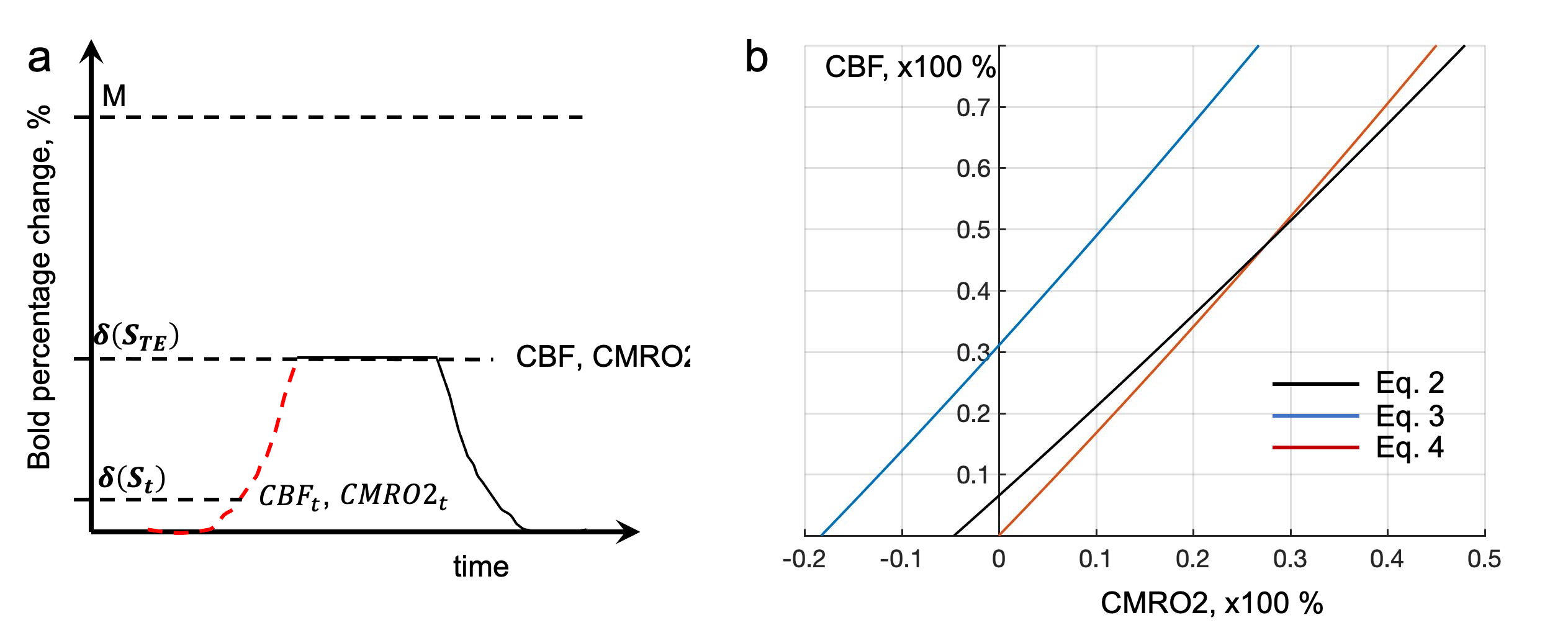
We define percentage change of variable L written as, δ(L)=L/L₀-1, where L and L₀ represent L at its activation and baseline states, respectively. Davis equation for relationship of fMRI signal and CBF and CMRO2 is shown as:$$\frac{CMRO2}{{CMRO2}_0}=\left(1-\frac{\delta\left(S_{TE}\right)}{M}\right)^{1/\beta}\left(\frac{CBF}{{CBF}_0}\mathrm{\ } \right)^{(1-\alpha/\beta)}(1),$$ where δ(S_TE) is BOLD signal percentage change; α and β are constants with approximate values of 0.38 and 1.5 (at task), respectively; M represents the maximum possible BOLD response. To derive governing relationship between δ(S_TE) and CBF changes, we need to introduce an auxiliary signal percentage of δ(S_t), which may be equal to δ(S_t)/ δ(S_TE)= δ(S_TE)/ M, as shown in Fig.1a. The CMRO2 changes with CBF can be written either relative to M as Eq. 2 (shown as black line in Fig.1b) or relative to δ(S_TE) as Eq. 3 (shown as blue line in Fig.1b). $$\delta\left(CMRO2_t\right)=\left(1-\frac{\delta\left(S_t\right)}{M}\right)^{1/\beta}\left(\frac{CBF_t}{{CBF}_0}\right)^{(1-\alpha/\beta)}-1 (2)$$ $$\delta\left(CMRO2\right)=\left(1-\frac{\delta\left(S_t\right)}{\delta\left(S_{TE}\right)}\right)^{1/\beta}\left(\frac{CBF}{{CBF}_0}\right)^{(1-\alpha/\beta)}-1. (3)$$ The change of CMRO2 relative to its baseline function can be written as Eq. (4) (shown as red line in Fig.1b), $$\delta\left(CMRO2\right)-\delta\left(CMRO2_0\right)=\left(1-\frac{\delta\left(S_t\right)}{\delta\left(S_{TE}\right)}\right)^{1/\beta}\delta\left(CBF'\right). (4)$$The Eq. 4 represents the changes CMRO2 relative to its baseline versus changes of δ(CBF’), where CBF’, a nominal CBF, is equal to (CBF)^(1-α/β), therefore, δ(CBF’)= (CBF/CBF₀)^(1-α/β)-1. The baseline function δ(CMRO2₀) is achieved by assigning CBF/CBF₀ equal to 1 in Eq. 3. Due to the cross point of Eq. 2 and Eq. 4 (black and red line in Fig. 1b), we can assign equal sign between right hand sides of Eq. 2 and Eq. 4 resulting Eq. 5 with the auxiliary signal change δ(S_t) being cancelled off after simplification and rearrangement. $$\delta\left(S_{TE}\right)=M\left(1-\frac{1}{\left(\frac{CBF}{{CBF}_0}\right)^{(1-\alpha/\beta)}}\right) (5)$$ Introducing Eq. 5 into Eq. 1 Davis equation, with the M being cancelled, we have final coupling relation between changes of CMRO2 and CBF shown as Eq. 6: $$\frac{CMRO2}{{CMRO2}_0}=\left(\frac{CBF}{{CBF}_0}\right)^n,\ n=\left(1-\frac{\alpha}{\beta}\right)\left(1-\frac{1}{\beta}\right). (6)$$ For the special case, when α=0.38 and β=1.5, we can have Eq. 7. $$\frac{CMRO2}{{CMRO2}_0}=\left(\frac{CBF}{{CBF}_0}\right)^{0.25}, (7)$$ where CMRO2/CMRO2₀=δ(CMRO2)+1 and CBF/CBF₀=δ(CBF)+1.

Results

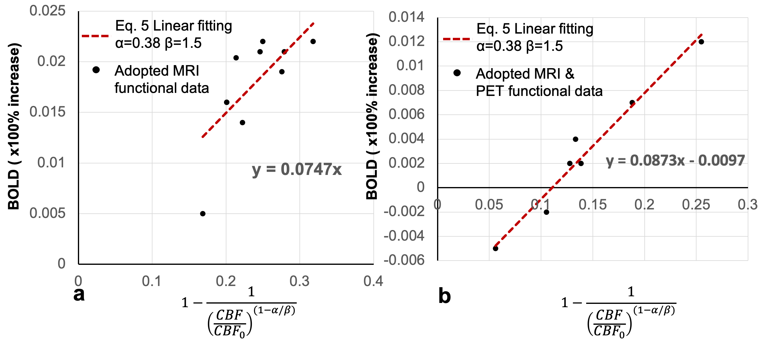
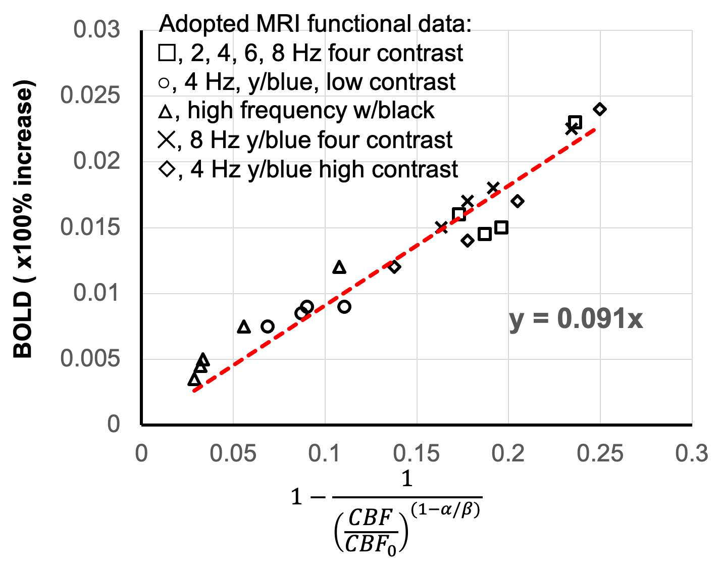
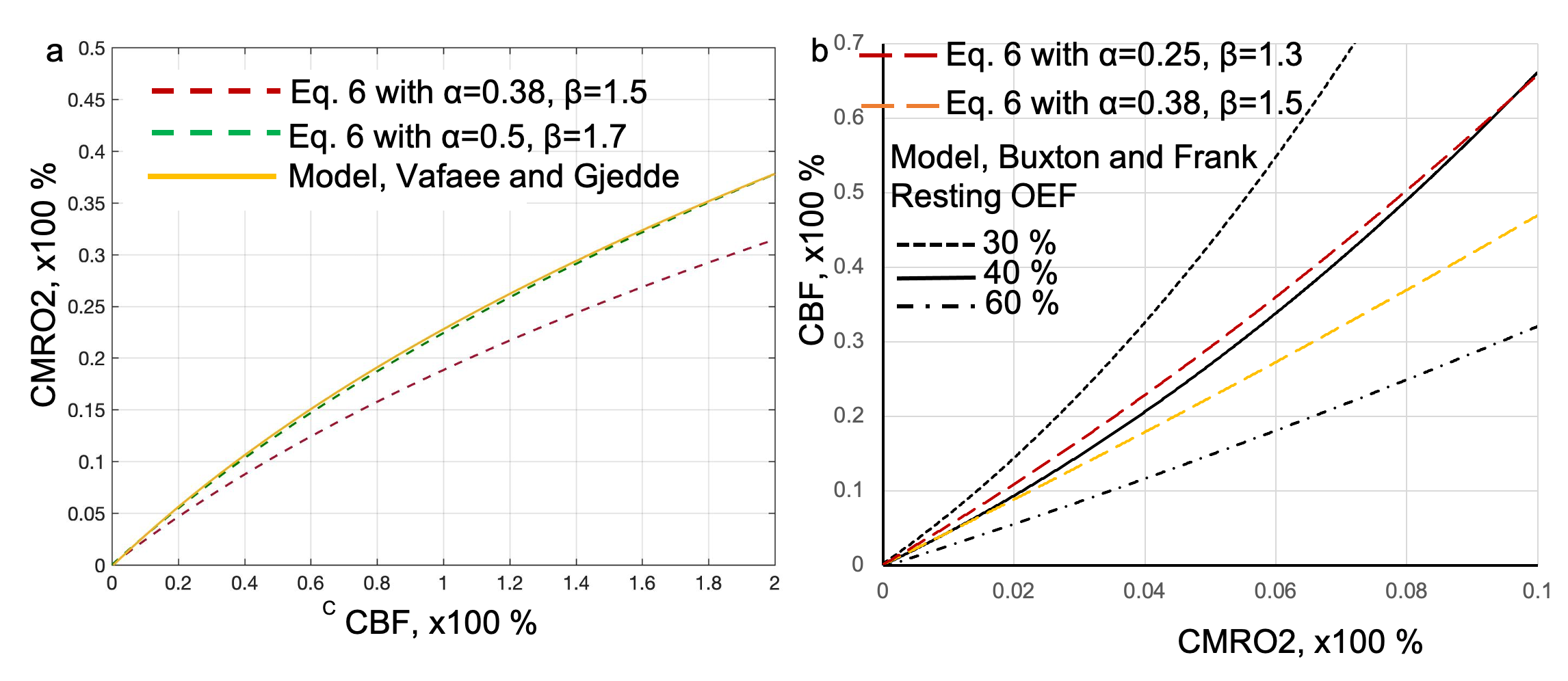
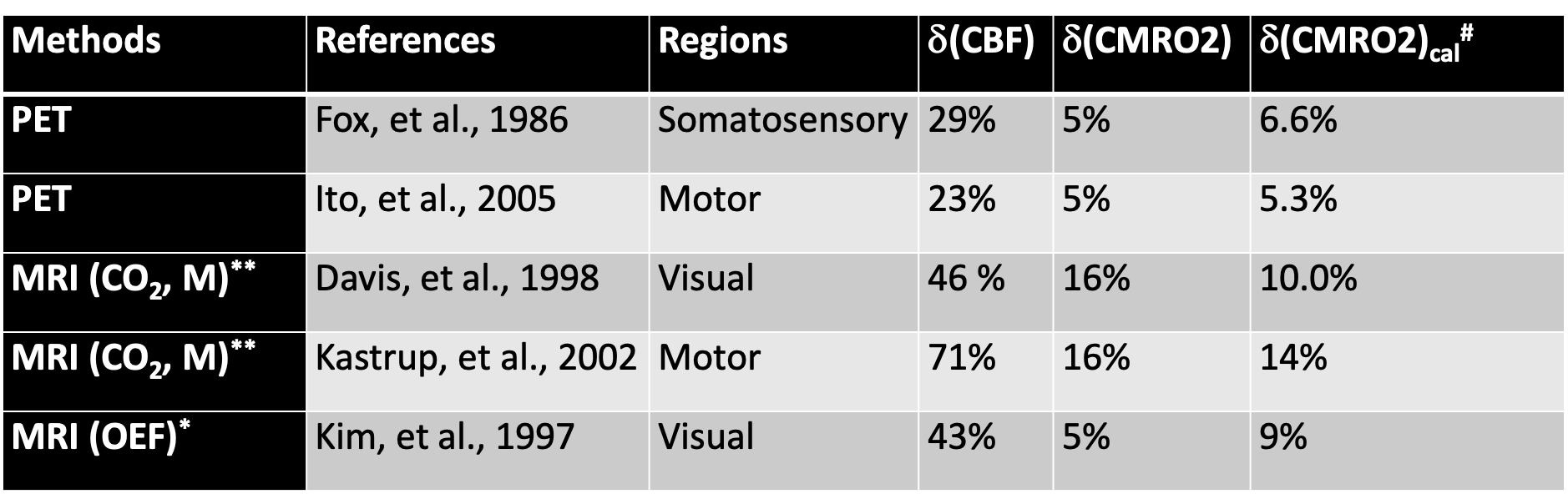
The Eq. 5 suggests that, when desired, M parameter can be measured directly from functional BOLD percentage change, δ(S_TE), and CBF functional changes instead of CO₂ calibration. We verify Eq. 5 by adapting CBF and BOLD functional stimulation datasets from two pioneering MRI works^[1,2] on Davis model and one PET_MRI dataset (PET for CBF measurement)^[5]. Results were shown in Fig. 2a, Fig. 3 and Fig. 2b, respectively, assuming a=0.38 and b=1.5. M parameters determined from linear fitting of Eq. 5 based on three functional datasets are approximately align with each other to around 0.08, which is generally accepted M in most of the previous measurements. It is worth to note that, in Fig. 3, there was a large discrepancy between fitted M-value of 0.09 and M-value of 0.22 based on CO2 calibration. It may suggest that M from CO₂ calibration may be sensitive to the experimental conditions. It is critical to verify Eq.5, which is the precondition for finalizing to Eq. 6, where M is cancelled off. Eq. 6 suggests changes of CMRO2 can be directly calculated from CBF without prior knowledge of M. In addition, Eq. 6 demonstrates a nonlinearity relationship of percentage change between δ(CBF) and δ(CMRO2). We compare Eq. 6 with two classical oxygen delivery models, ^[3,4] in Fig. 4a and Fig. 4b, respectively. We show the nonlinearity of Eq. 6 is comparable with both models. When CBF change is small, percentage change between δ(CBF) and δ(CMRO2) in Eq. 6 can be linear by Taylor expansion. In that case, n in Eq.6, approximately equal to n=0.25~0.33, (assuming α=0.38~0.56), is equivalent to conventional coupling constant n_c=3~4, which is in line with previously reported n_c=2~4.The references of previously reported δ(CMRO2) vary significantly based on different techniques, brain regions and stimulation types. We compare some previously reported δ(CMRO2) with the calculated δ(CMRO2)_cal based on Eq.7 (introducing correspondingly reported δ(CBF) in these works into Eq. 7). The result is shown in Table. 1, where our calculation results δ(CMRO2)_cal are approximately in line with reported δ(CMRO2).

Conclusions

We demonstrate M parameter can be measured directly from BOLD and CBF functional changes instead of CO₂ calibration. We show that percentage changes of δ(CMRO2) can be directly calculated from δ(CBF) changes without prior knowledge of M. Comparing with two classical models, we show the nonlinearity between δ(CMRO2) and δ(CBF) is comparable to two classical models. The calculations of percentage changes, δ(CMRO2)_cal, based on our equation, are approximately consistent with previous results reported from both PET and MRI.

Acknowledgements

This work was supported by the Intramural Research Program of the National Institute of Mental Health, USA. Thanks for productive discussion with Dr. Nicholas Blockley from University of Nottingham.