3385
Optimizing EEG source reconstruction with concurrent fMRI-derived spatial priors1Coimbra Institute for Biomedical Imaging and Translational Research (CIBIT), Institute for Nuclear Sciences Applied to Health (ICNAS), University of Coimbra, Coimbra, Portugal, 2Neurology Department, Centro Hospitalar e Universitário de Coimbra, Coimbra, Portugal, 3Faculty of Medicine, University of Coimbra, Coimbra, Portugal
Synopsis
There is no consensus regarding the optimal EEG source reconstruction algorithm, nor a systematic comparison between sets of fMRI-derived spatial priors to be included in the inversion models. We compared four inversion algorithms, each with three sets of fMRI-derived spatial priors consisting of task activation maps, resting-state networks and, for the first time, dynamic functional connectivity states. We found that combining a beamformer with these priors improves the reconstruction quality, especially in terms of the overlap with task-related brain regions of interest and RSN templates. Our results may guide more informatively the selection of the optimal EEG source reconstruction approach.
Introduction
Reconstructing EEG sources involves a complex pipeline1,2, with the inverse problem being the most challenging due to the non-uniqueness of its solution, which can be partially circumvented by including fMRI-derived spatial priors in the inverse models3. However, only task activation maps and resting-state networks (RSNs) have been explored so far, overlooking the notion that brain networks exhibit dynamic functional connectivity (dFC) fluctuations4. Moreover, there is no consensus regarding the inversion algorithm of choice, nor a systematic comparison between different sets of spatial priors. Using simultaneous EEG-fMRI data, here we compared four different inversion algorithms, each with three different sets of priors (or covariance components, CCs) under a Parametric Empirical Bayesian framework5.Methods
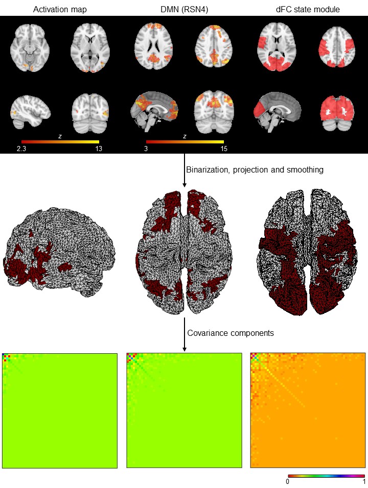
Data acquisition and pre-processing: Six patients with Multiple Sclerosis and seven demographically matched healthy subjects were studied on a 3T MRI system (Siemens) using an MR-compatible 64-channel EEG system (NeuroScan). BOLD-fMRI (2D-EPI, TR/TE=1000/37ms, 2mm isotropic) was acquired concurrently with EEG during four runs of: an hMT/V5+ functional localizer6 (3.2min), two biological motion perception7 (8.4min), and resting-state (8min). EEG data were MR-induced artifact corrected8,9, band-pass filtered (1-30Hz), and further pre-processed10, as well as fMRI data11.fMRI-derived CCs (Fig. 1): First, task activations were mapped using a GLM with regressors marking the stimulation periods, followed by cluster thresholding (voxel Z>2.5, cluster p<0.05)12. Second, spatial ICA decomposition13 was performed for each run and participant, identifying 10 RSNs based on their spatial overlap (quantified by the Dice coefficient14) with RSN templates15. Third, dFC was computed from parcel-averaged BOLD signals across AAL-based regions16 with a phase coherence approach17, followed by a l1-regularized dictionary learning step for extracting the dFC states18. By correlating their contribution over time to the overall dFC with the task regressors, task-related dFC states were determined, and network modules were obtained using the Louvain algorithm19. These 3D maps were then binarized, projected onto the 2D cortical surface5, and smoothed using the Green’s function20. The CCs of the resulting 2D spatial priors were obtained as their outer product.
EEG source reconstruction (Fig. 2): The forward problem was solved with: 1) realistic head models from the segmentation of the structural images into 6 tissues; 2) electrode positions manually adjusted to match the distortions on the structural images; and 3) volume conduction models built using boundary element models. EEG data was downsampled to 60Hz and reconstructed at each time point considering four algorithms (minimum norm, MN21; low-resolution electromagnetic tomography, LORETA22; empirical Bayes beamformer, EBB23; and multiple sparse priors, MSP24), each with three different sets of CCs consisting of: S1) those specific to the algorithm; S2) S1 plus RSNs and task activation maps; and S3) S2 plus task-related dFC state modules. Reconstruction quality was assessed in terms of the free-energy (FE) and variance explained (VE) of the inversion models, and the overlap (quantified by the Dice coefficient d) of RSN templates and atlas-based anatomical brain regions known to be involved in similar tasks7, with EEG source components obtained by applying spatial ICA to the reconstructed EEG. The main effects of the population group, inversion algorithm and set of CCs were evaluated by a 3-way ANOVA for each quality metric separately, with subsequent post-hoc statistical tests (p<0.05).
Results
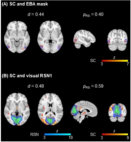
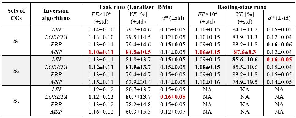
Fig. 3 shows a considerable overlap of two EEG source components with an extrastriate body area mask (EBA; known to be involved in similar tasks7) and a visual RSN template. No differences were found between population groups for any metric. Table 1 depicts the average FE, VE and d values across participants, and across task runs. For the FE and VE values, there was no main effect of the algorithm, while S1 was significantly better than S2 and S3. The combination MSP+S1 yielded the lowest/highest FE/VE for all runs, performing significantly better than other five combinations using sets S2 or S3. In contrast, LORETA+S3 and EBB+S2 achieved the highest d for the task and resting-state runs, respectively. The post-hoc tests of the d values revealed that: MN and EBB performed significantly better than LORETA and MSP, using the sets S2 and S3 was significantly better than set S1, and EBB+S2 exhibited significantly higher d than combinations with MN or LORETA, and S1.Discussion and Conclusion
We found that including fMRI-derived spatial priors critically improves the quality of EEG source reconstruction, with no differential effect between groups. The usefulness of this type of priors have already been reported5,25–28, although the resulting reconstructions were only compared using conventional quality metrics. According to the d values, we found that LORETA performed significantly worse than MN or EBB, suggesting that the low-resolution (smoothed) solutions of LORETA may render it inappropriate for localizing such specific sources as those involved in the tasks1. This is in line with previous comparison studies on simulated data29–32. The post-hoc analysis revealed that dFC states convey relevant information for EEG reconstruction on the task runs (S3), and that EBB+S2 exhibited the best d values; the latter suggests that by coupling inversion algorithms as beamformers designed for providing focal solutions with fMRI-derived information, an optimal balance between sensitivity and specificity is achieved. We believe that such recommendations based on our analyses may more informatively guide the selection of the optimal EEG reconstruction approach.Acknowledgements
This work was supported by Grants Funded by Fundação para a Ciência e Tecnologia, PAC –286 MEDPERSYST, POCI-01-0145-FEDER-016428, BIGDATIMAGE, CENTRO-01-0145-FEDER-000016 financed by Centro 2020 FEDER, COMPETE, FCT UID/4950/2020 – COMPETE, CONNECT.BCI POCI-01-0145- FEDER-30852, and BIOMUSCLE PTDC/MEC-NEU/31973/2017. FCT also funded an individual grant to JVD (Individual Scientific Employment Stimulus 2017 - CEECIND/00581/2017).References
1. Michel, C. M. & Murray, M. M. Towards the utilization of EEG as a brain imaging tool. Neuroimage 61, 371–385 (2012).
2. Michel, C. M. & Brunet, D. EEG source imaging: A practical review of the analysis steps. Front. Neurol. 10, (2019).
3. Lei, X., Wu, T. & Valdes-Sosa, P. A. Incorporating priors for EEG source imaging and connectivity analysis. Front. Neurosci. 9, 284 (2015).
4. Preti, M. G., Bolton, T. A. & Van De Ville, D. The dynamic functional connectome: State-of-the-art and perspectives. Neuroimage 160, 41–54 (2017).
5. Henson, R. N., Flandin, G., Friston, K. J. & Mattout, J. A Parametric empirical bayesian framework for fMRI-constrained MEG/EEG source reconstruction. Hum. Brain Mapp. 31, 1512–1531 (2010).
6. Huk, A. C., Dougherty, R. F. & Heeger, D. J. Retinotopy and functional subdivision of human areas MT and MST. J. Neurosci. 22, 7195–7205 (2002).
7. Chang, D. H. F., Ban, H., Ikegaya, Y., Fujita, I. & Troje, N. F. Cortical and subcortical responses to biological motion. Neuroimage 174, 87–96 (2018).
8. Allen, P. J., Josephs, O. & Turner, R. A method for removing imaging artifact from continuous EEG recorded during functional MRI. Neuroimage 12, 230–239 (2000).
9. Abreu, R. et al. Ballistocardiogram artifact correction taking into account physiological signal preservation in simultaneous EEG-fMRI. Neuroimage 135, 45–63 (2016).
10. da Cruz, J. R., Chicherov, V., Herzog, M. H. & Figueiredo, P. An automatic pre-processing pipeline for EEG analysis (APP) based on robust statistics. Clin. Neurophysiol. 129, 1427–1437 (2018).
11. Abreu, R., Nunes, S., Leal, A. & Figueiredo, P. Physiological noise correction using ECG-derived respiratory signals for enhanced mapping of spontaneous neuronal activity with simultaneous EEG-fMRI. Neuroimage 154, 115–127 (2017).
12. Woolrich, M. W., Ripley, B. D., Brady, M. & Smith, S. M. Temporal autocorrelation in univariate linear modeling of FMRI data. Neuroimage 14, 1370–86 (2001).
13. Beckmann, C. F. & Smith, S. M. Probabilistic independent component analysis for functional magnetic resonance imaging. IEEE Trans. Med. Imaging 23, 137–52 (2004).
14. Dice, L. R. Measures of the Amount of Ecologic Association Between Species. Ecology 26, 297–302 (1945).
15. Smith, S. M. et al. Correspondence of the brain’s functional architecture during activation and rest. Proc. Natl. Acad. Sci. U. S. A. 106, 13040–13045 (2009).
16. Tzourio-Mazoyer, N. et al. Automated Anatomical Labeling of Activations in SPM Using a Macroscopic Anatomical Parcellation of the MNI MRI Single-Subject Brain. Neuroimage 15, 273–289 (2002).
17. Cabral, J. et al. Cognitive performance in healthy older adults relates to spontaneous switching between states of functional connectivity during rest. Sci. Rep. 7, 1–13 (2017).
18. Abreu, R., Leal, A. & Figueiredo, P. Identification of epileptic brain states by dynamic functional connectivity analysis of simultaneous EEG-fMRI: a dictionary learning approach. Sci. Rep. 9, 638 (2019).
19. Rubinov, M. & Sporns, O. Complex network measures of brain connectivity: Uses and interpretations. Neuroimage 52, 1059–1069 (2010).
20. Harrison, L. M., Penny, W., Ashburner, J., Trujillo-Barreto, N. & Friston, K. J. Diffusion-based spatial priors for imaging. Neuroimage 38, 677–695 (2007).
21. Hämäläinen, M. S. & Ilmoniemi, R. J. Interpreting magnetic fields of the brain: minimum norm estimates. Med. Biol. Eng. Comput. 32, 35–42 (1994).
22. De Peralta-Menendez, R. G., Murray, M. M., Michel, C. M., Martuzzi, R. & Gonzalez Andino, S. L. Electrical neuroimaging based on biophysical constraints. Neuroimage 21, 527–539 (2004).
23. López, J. D., Litvak, V., Espinosa, J. J., Friston, K. & Barnes, G. R. Algorithmic procedures for Bayesian MEG/EEG source reconstruction in SPM. Neuroimage 84, 476–487 (2014).
24. Friston, K. et al. Multiple sparse priors for the M/EEG inverse problem. Neuroimage 39, 1104–1120 (2008).
25. Lei, X., Hu, J. & Yao, D. Incorporating fMRI functional networks in EEG source imaging: A bayesian model comparison approach. Brain Topogr. 25, 27–38 (2012).
26. Lei, X., Qiu, C., Xu, P. & Yao, D. A parallel framework for simultaneous EEG/fMRI analysis: Methodology and simulation. Neuroimage 52, 1123–1134 (2010).
27. Lei, X. et al. fMRI functional networks for EEG source imaging. Hum. Brain Mapp. 32, 1141–1160 (2011).
28. Lei, X. Electromagnetic brain imaging based on standardized resting-state networks. in 2012 5th International Conference on Biomedical Engineering and Informatics, BMEI 2012 40–44 (2012).
29. Bradley, A., Yao, J., Dewald, J. & Richter, C. P. Evaluation of electroencephalography source localization algorithms with multiple cortical sources. PLoS One 11, 1–14 (2016).
30. Halder, T., Talwar, S., Jaiswal, A. K. & Banerjee, A. Quantitative evaluation in estimating sources underlying brain oscillations using current source density methods and beamformer approaches. eNeuro 6, 1–14 (2019).
31. Yao, J. & Dewald, J. P. A. Evaluation of different cortical source localization methods using simulated and experimental EEG data. Neuroimage 25, 369–382 (2005).
32. Grova, C. et al. Evaluation of EEG localization methods using realistic simulations of interictal spikes. Neuroimage 29, 734–753 (2006).
Figures
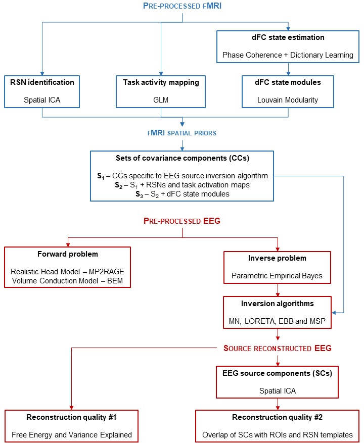
Fig. 1: Schematic diagram of the processing pipeline. Three types of fMRI spatial priors for EEG source reconstruction are extracted: 1) RSNs through spatial ICA; 2) task-related activity maps through GLM; and 3) network modules from task-related dFC states. The CCs associated with these spatial priors were then included in several inversion algorithms, whose reconstruction quality was assessed by the FE, VE and overlap of EEG source components with ROIs and RSN templates.