Introduction

Simultaneous EEG-fMRI acquisitions are used to exploit their highly complementary characteristics of the two modalities, and this is of potential interest for neurofeedback (NF) applications. While EEG is not only inexpensive but also portable and easy to operate, fMRI is able to capture the activity of target brain areas or networks with much higher specificity. This complementarity has motivated the search for solutions capable of identifying EEG models that predict a given fMRI signal of interest, based on simultaneous EEG-fMRI recordings, so that appropriate EEG-based NF protocols can then be developed^1,2,3. The default mode network (DMN) has been robustly identified in resting-state fMRI studies and found to be impaired in several disorders. Although NF protocols targeting the DMN are therefore of special interest, the corresponding EEG features have not been identified. Here we investigate an integration strategy whereby relevant EEG features are extracted and linear models are learnt so as to predict the DMN activity measured by simultaneous fMRI.

Methods

Concurrent EEG-fMRI data was acquired from 6 episodic migraine patients without aura in the interictal phase, on a Siemens 3T MR scanner, during a session of 7 min eyes-open resting state. fMRI was acquired with a gradient-echo 2D-EPI sequence (TR/TE=1260/30ms, 2.2mm isotropic resolution, SMS-3 and in-plane GRAPPA-2). EEG data was acquired with a MR-compatible 32-channel EEG system (Brain Products), sampled at 1kHz.

fMRI data underwent distortion correction and motion correction, followed by ICA-FIX cleanup (FSL⁴). The average cerebrospinal fluid and white matter signals, along with motion parameters and outliers, were regressed out. The resulting data was high-pass filtered (cut-off 0.01Hz) and spatially smoothed (FWHM=3.3mm). A second ICA procedure was performed at the subject level to extract putative subject specific resting state networks. The DMN IC was identified by template matching based on a reference DMN⁵, and its time-series was extracted as the fMRI signal of interest. Prior to model estimation, it was up-sampled at 4Hz and normalized.

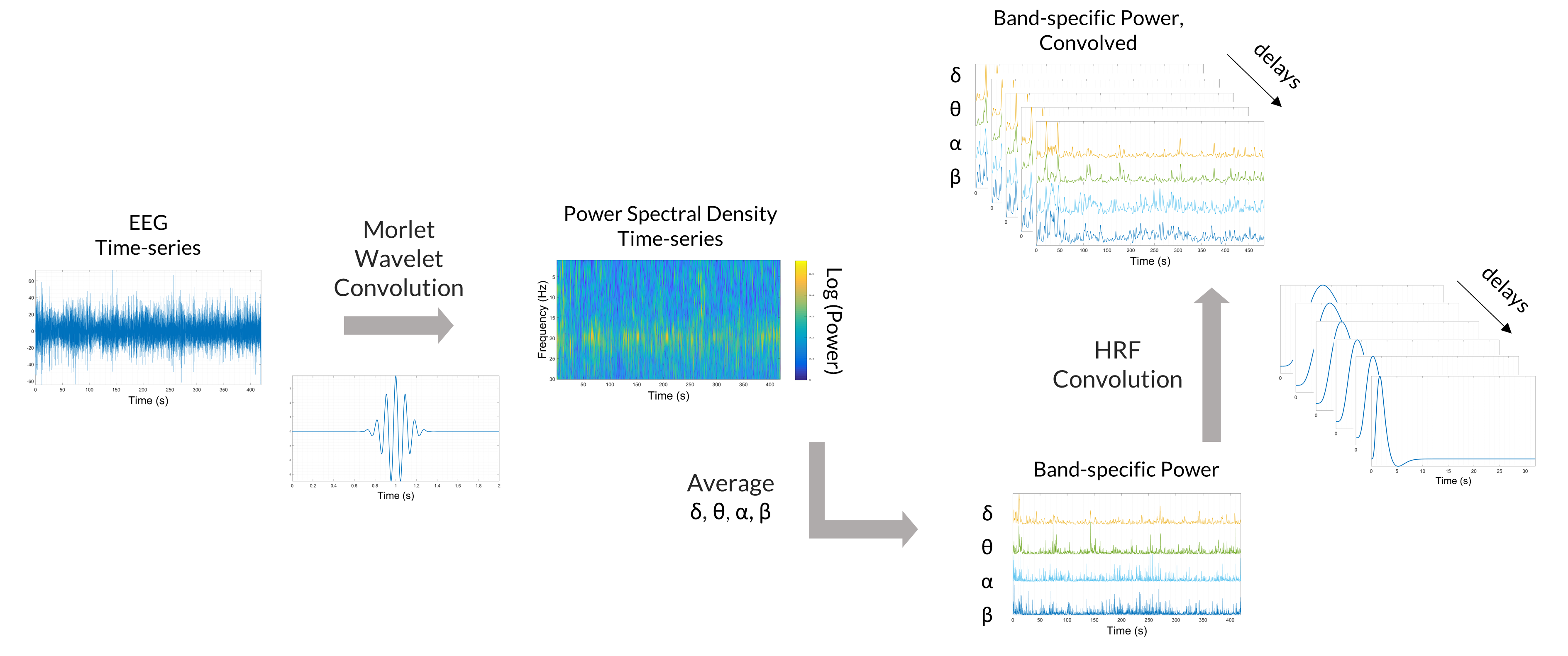
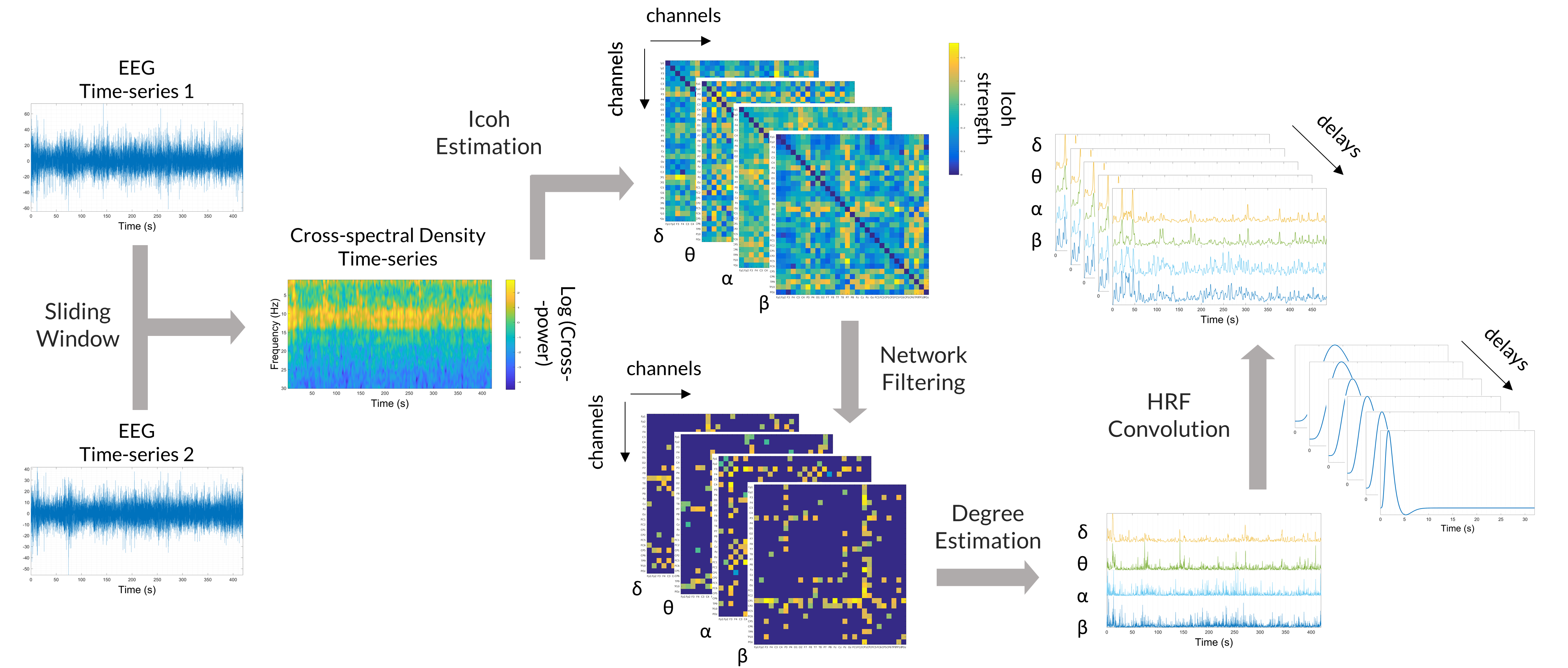
EEG data underwent gradient artifact correction, was down-sampled at 250Hz, and corrected for the pulse artifact. Signals were then band-pass filtered (0.5-40Hz), re-referenced and ICA-denoised (EEGLAB⁶, Matlab). From the EEG spectrum and cross-spectrum, the following spectral and coherence features were derived for each channel, as possible models of the linear relationship between EEG activity and the BOLD signal: root mean squared frequency (RMSF), total power (TP), linear combination of band-specific EEG power (LC) (Fig.1), and weighted degree of the functional connectivity network built from the band-specific imaginary part of coherency of the EEG cross-spectrum (WD-ICoh) (Fig.2). The following frequency bands were considered: for δ (1-4Hz), θ (4-8Hz), α (8-12Hz), β (12-30Hz).
Each EEG feature was convolved with a 32s hemodynamic response function (HRF), modelled by the combination of two gamma functions. To accommodate for the variability of the HRF, each EEG feature was convolved with a set of different HRFs, with overshoot delays of 10,8,6,5,4 and 2s. The resulting features were down-sampled at 4Hz and normalized.

Each EEG predictor model (RMSF, TP, LC, WD-Icoh) was fitted to the fMRI DMN signal independently by linear regression, using the elastic net regularization (ENR) method, which incurs a mixed L₁₂ penalty on the least-squares objective function⁷. Regularization was used to reduce model complexity so as to improve model interpretability and control for overfitting effects. ENR requires the specification of two hyperparameters prior to model estimation: the λ parameter (ratio between the weights of the L₁ and the L₂ penalty), and a complexity parameter, α. To keep computational cost to a minimum, α was set to 0.6 in all analyses, whilst λ was optimized. A nested k-fold CV procedure (k=15 outer folds, m=10 inner folds), was used for both model selection (inner CV) - optimization of the λ parameter - and evaluation (outer CV) - estimation of the prediction error and other criteria of model performance. The Bayesian information criterion (BIC)⁹, designed to balance goodness-of-fit and model simplicity, was used for model selection.

Measures of performance, estimated in the test sets of all CV folds and subjects, were compared between models through analysis of variance (ANOVA, Matlab)

Results

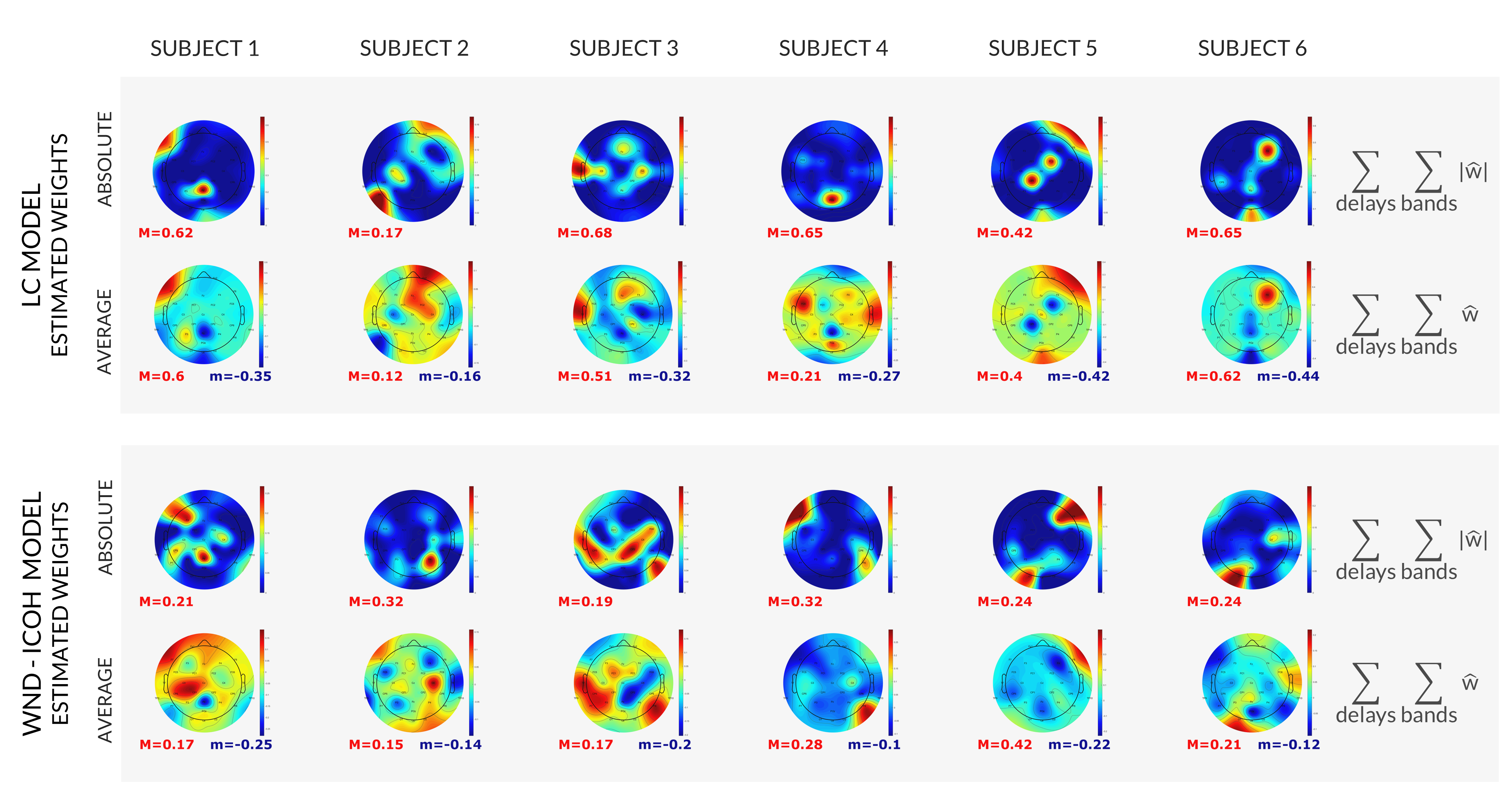
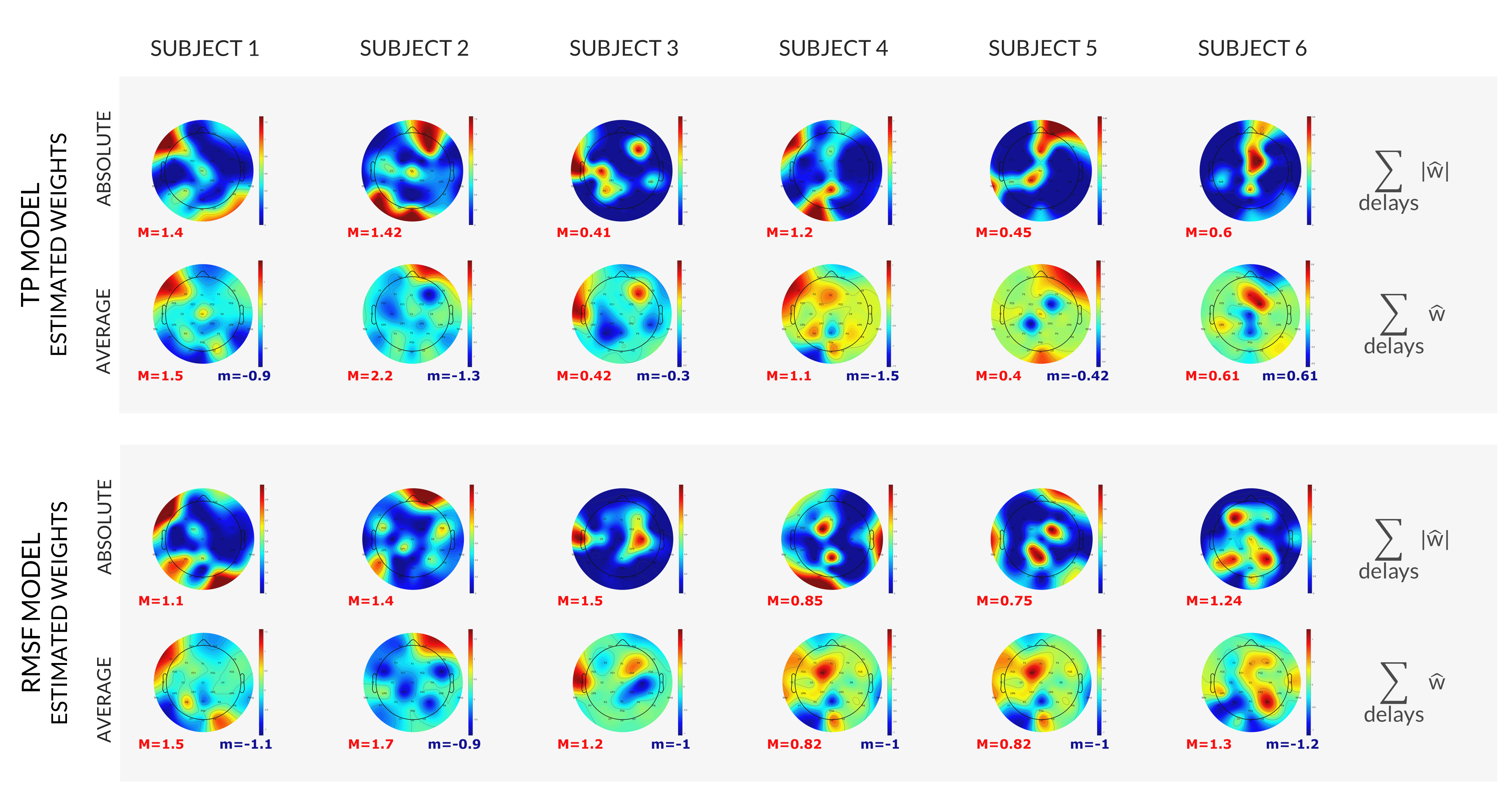
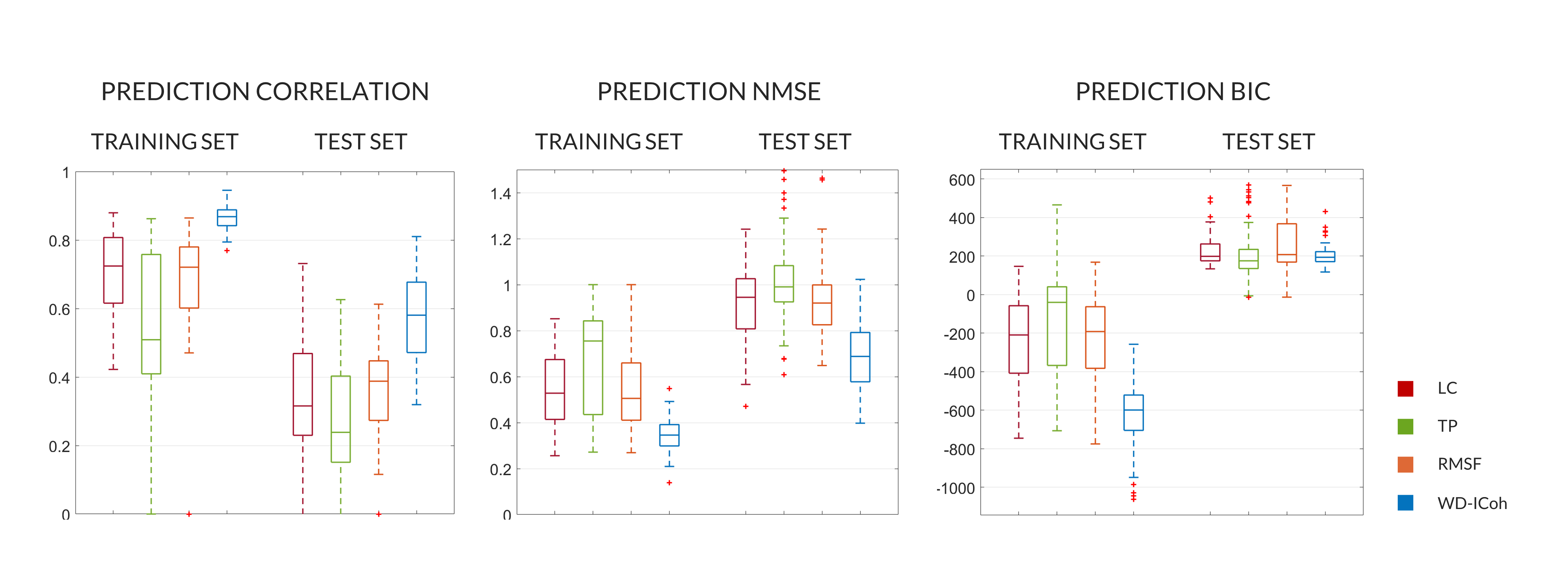
The estimated models are presented in Figures 3-4, where the importance of each channel to the final model is shown.
ANOVA results are reported in Figure 5. Similarity between the predicted and original BOLD time-series was assessed by the Pearson's correlation coefficient and the normalized mean squared error. Both were significantly better (p-values 7.75e-8 to 3.77e-9) for the WN-Icoh model than for all the remaining models. Correlation was also significantly lower for the TP models than for all the remaining models (p-values 3.38e-3 to 3.77e-9). BIC was significantly better for the TP and WN-ICoh models than for the RMSF model (p-values 3.82e-2, 3.37e-2), which indicates that the models with worse goodness-of-fit are compensating by using less features to predict the target signal.

Discussion and Conclusion

The models here developed were able to predict the target BOLD signal from the DMN with fairly good correlations (mean 0.25-0.58, median 0.24-0.58).
Our results indicate the viability of the proposed EEG models in predicting the simultaneous fMRI signal from the DMN. We also showed that measures of similarity between the predicted and target BOLD signal significantly varied with the model used.

Acknowledgements

We acknowledge the Portuguese Science Foundation through grants PTDC/EMD-EMD/29675/2017, LISBOA-01-0145-FEDER-029675 and UIDB/50009/2020.