INTRODUCTION

NIST and the ISMRM ad-hoc Committee on Standards for Quantitative Magnetic Resonance, designed and commercialized a standard MRI system phantom^1,2 to assess scanner performance, stability, inter-comparability and accuracy of quantitative relaxation time imaging^3-5. Several important measurement protocols need to be improved and made more rigorous. The items addressed here are: 1) using the embedded liquid crystal (LC) MR-visible thermometer⁶ to automatically record phantom temperature; 2) ascertaining efficacy of geometric distortion corrections; and 3) determining the effects of the fill conductivity on the MR measurements.

METHODS

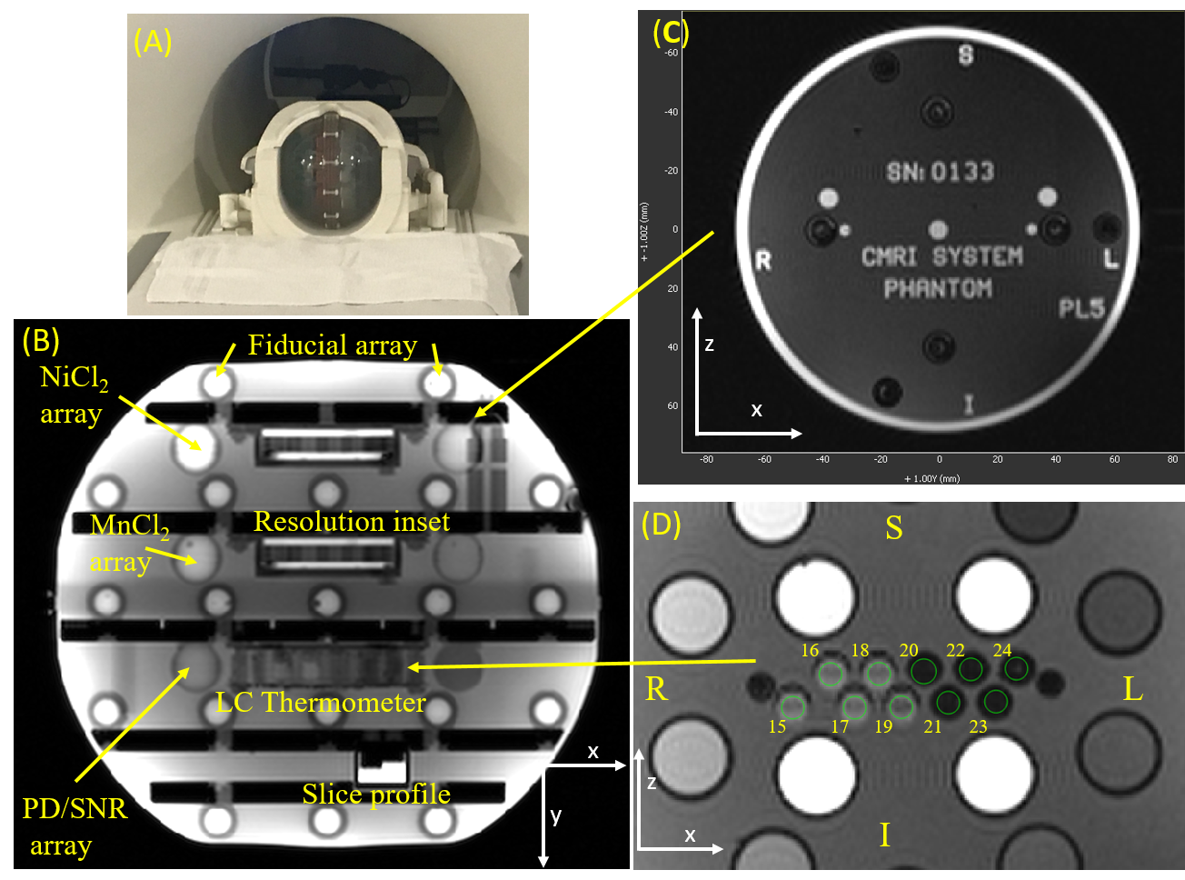
Two commercial MRI system phantoms were purchased⁷, along with reference solutions. The solution T1, T2 relaxation times were traceably calibrated at 3T over a temperature range from 16C to 26C. Geometric accuracy was calibrated using traceable CT. The system phantoms are included in the NIST/ NIBIB phantom lending library https://www.nist.gov/programs-projects/nistnibib-medical-imaging-phantom-lending-library and are available for check-out. The phantoms were characterized on a 3T scanner using a 32-channel head coil with the plates in the sagittal plane (Figure 1A), a 90° rotation of the phantom from its default orientation. All data were analyzed using an open-source package PhantomViewer (https://github.com/MRIStandards/PhantomViewer). The LC thermometer consists of 10 cylindrical cells with transition temperatures varying in 1C increments from 15C to 24C. Circular 4mm diameter regions of interest were used to collect signal data for thermometry. Geometric distortion analysis was done by fitting the fiducial array, consisting of 56 precisely-machined 10.0mm spheres on a 40.0mm grid (1). The phantoms were imaged with both a deionized water fill and a phosphate-buffered saline fill with 20C conductivities of < 10^-4S/m and 0.43S/m, respectively. The saline conductivity was chosen to be comparable to the conductivity of human tissue.

RESULTS

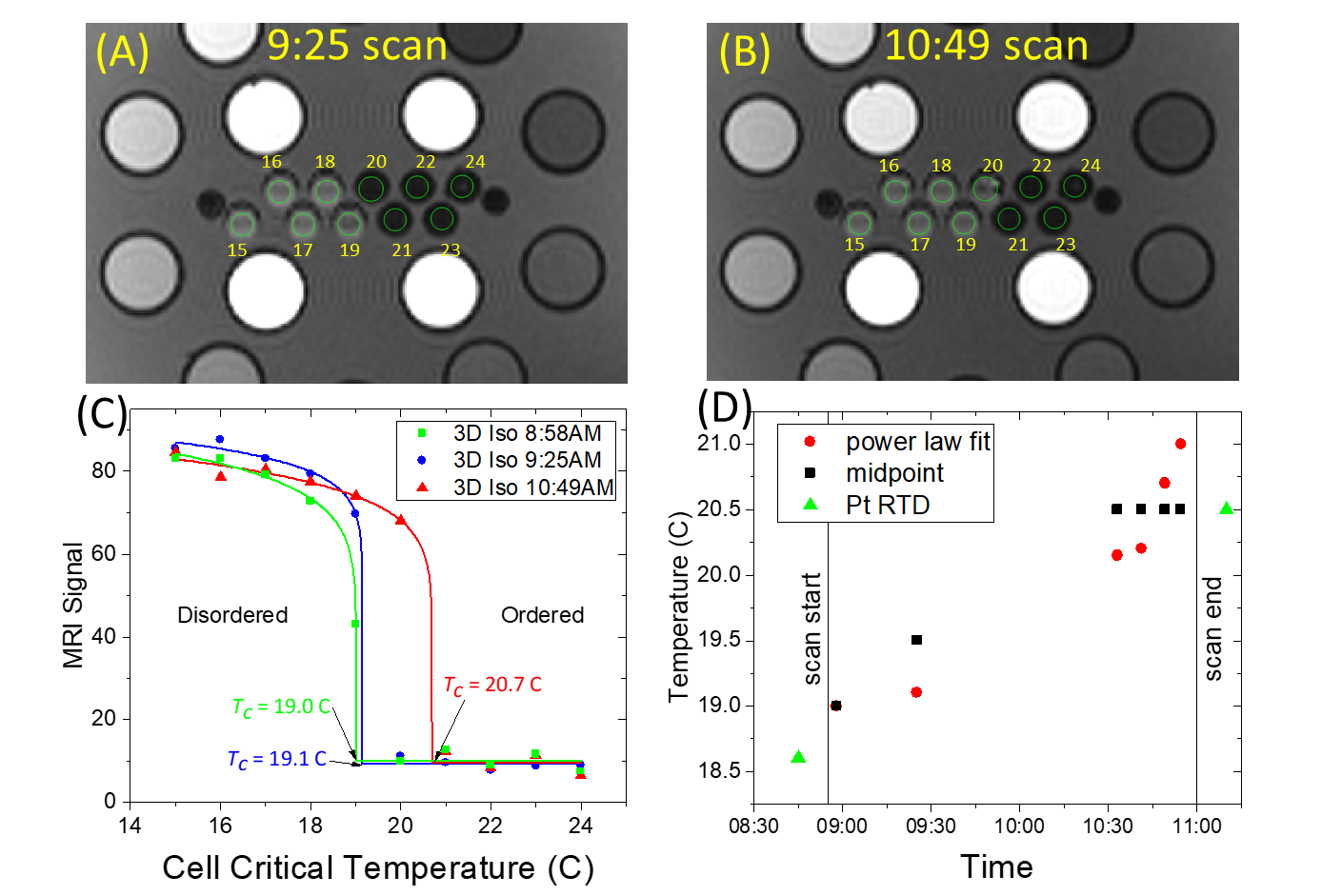
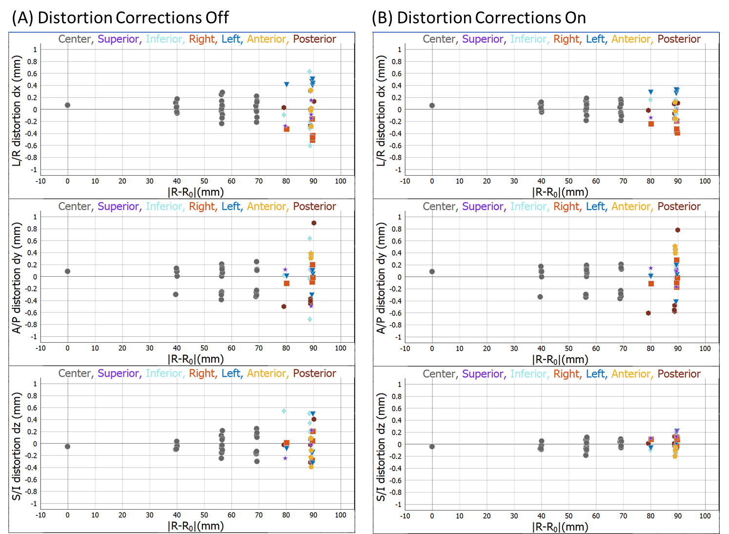
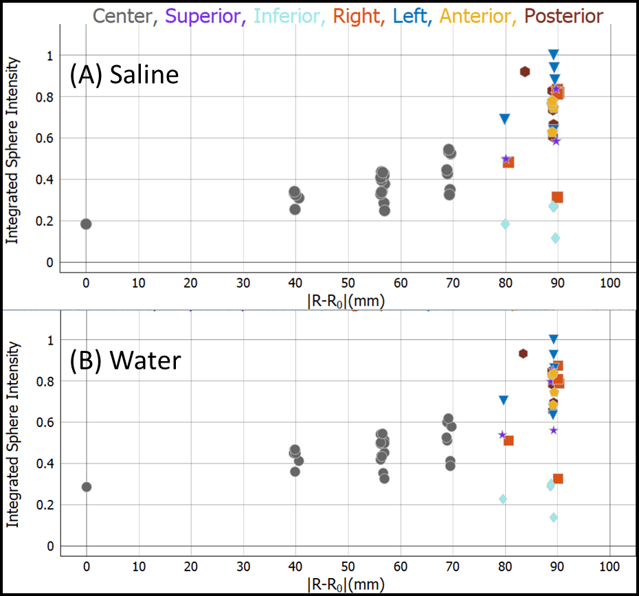
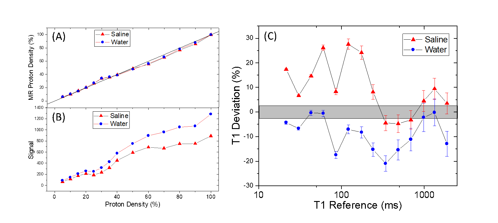
Figure 1 B,C,D show the system phantom configuration, the top plate with serial number, and the LC thermometer. The LC thermometer shows bright/dark cells where the LC critical temperatures are below/above the phantom temperature, respectively. The on-cells have a small ~ 1mm chemical shift artifact along the frequency-encode direction. Figure 2A,B show the LC thermometer at two points during the scanning session indicating the phantom is warming. Figure 2C shows the MR signal for each cell for three isotropic 3D scans taken at different times during the imaging session. The temperature can be determined by using a power law fit to the data, or by manually taking the midpoint between the last on-cell and the first off-cell critical temperature. These phantom temperatures are shown in Fig. 2D along with Pt-resistance thermometer measurements. Figure 3A,B show geometric distortion, defined as the difference of the apparent position of each fiducial sphere from the real position, obtained from a 3D GRE scan with and without software-based distortion corrections. The scans were done in the plane of the phantom plates, with the y-direction being perpendicular to the plates and scan plane. The software correction improves the in-plane distortion to < ±0.4mm and < ±0.2mm perpendicular and parallel to the scanner bore, respectively. The distortion correction applied here did not correct for the out of plane distortions. The change in fill causes a small shift in the image signal distribution across the phantom (Figure 4), with signal loss in the center of the phantom for the saline fill. A change in MR signal can also be observed for the proton density array (Figure 5) for the saline and water fills. The primary measurement, MR proton density, where the signal is normalized to the local background signal is not strongly affected. The biggest effect of the fill conductivity was observed in the variable flip angle (VFA) T1 protocol (Figure 5C). VFA is sensitive to nonuniformities in the RF transmit field which will be a function of the electromagnetic properties of the phantom fill. Other effects, including prescan shimming and RF power transmit/receive gains may have important effects which may lead to much greater variability in VFA.

DISCUSSION

The MR-readable thermometer allows the temperature to be embedded in the MR data at scan time and provides a more reliable method of recording phantom temperature. The thermometer accuracy is ±0.5C, which is sufficient to push the thermal uncertainty for T1, T2 measurements on the NiCl₂ array below 2%. The geometric distortion measurements are quick and useful ways to understand the intrinsic scanner accuracy due to nonuniform gradients as well as to verify that the software corrections are adequate. Figure 3B shows that current scanners can have geometric distortion less than 1 part in 10³, hence calibration standards must exceed this accuracy. The effect of fill has a small effect on primary measurements but may have a considerable effect on less robust protocols such as T1 VFA. The effect and optimization of the electromagnetic properties of the phantom fill need to be further explored.

CONCLUSION

Here we describe improvements and applications of the MRI system phantom including the incorporation of an MR-readable thermometer, simple evaluation of scanner geometric distortion and efficacy of distortion corrections, and the effect of varying the electromagnetic properties of the fill solution. While the MRI system phantom has limitations and considerable complexity, it provides necessary information and validation for many types of quantitative measurements.

Acknowledgements

We thank all of the members of the ISMRM SQMR committee for input and guidance. We thank Nikki Rentz for long hours doing traceable NMR calibrations.