Introduction

Imperfections of the gradient system transfer function (GSTF) often degrade the quality of reconstructed images due to distortion of the k-space trajectory. To suppress degradation of images, techniques have been proposed including measurement of GSTF¹ and pre-emphasis of gradients using GSTF². Existing studies represented the GSTF using either infinite impulse response (IIR) filters³ using approximation methods⁴ or filters in the Fourier domain. Finite impulse response (FIR) filters with a large number of taps can represent arbitrary GSTF since practical filters with feedback terms become zero at a certain precision of floating-point operations (e.g. 32-bit float). While FIR filters are usually not considered to represent the GSTF, they have good properties such as numerical stability and capability of stream processing. The only drawback of FIR filters is their computational complexity. In this work, the author proposes a new representation of GSTF based on FIR filters. Because FIR filters can represent arbitrary functions, the author expects that the proposed representation covers various composite functions that come from both physical GSTF and vendor-specific black-box circuits.

Theory

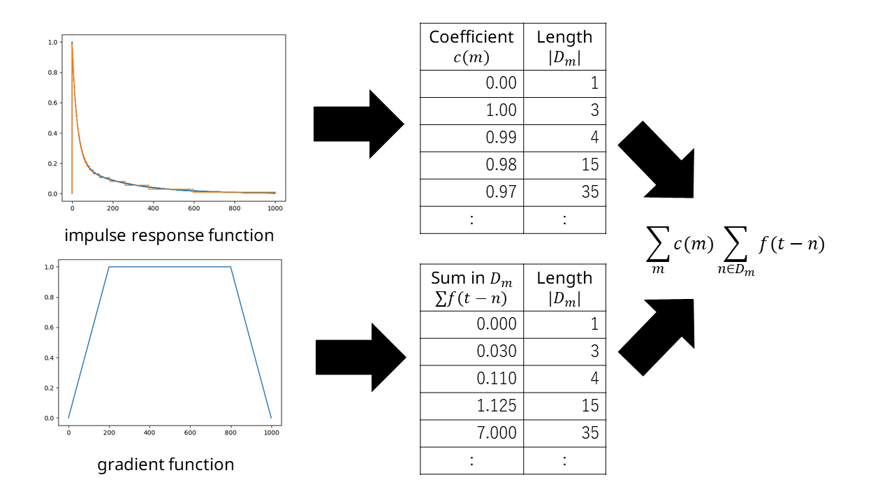
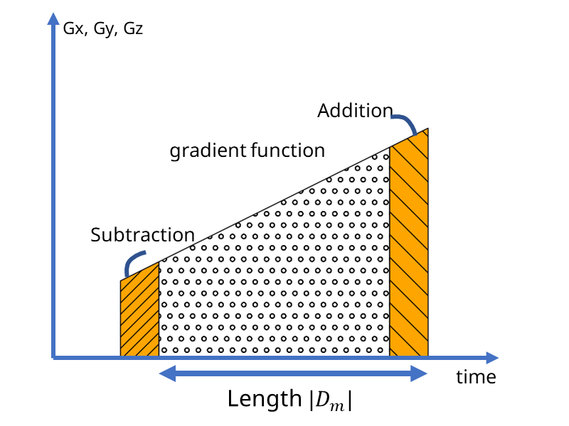
An $$$N$$$-tap FIR filter for time $$$t \in \mathbb{Z}$$$ can be represented as $$g(t)=\sum_{n=0}^{N-1}a(n)f(t-n)$$ where $$$a(n)$$$ , $$$f(t)$$$ and $$$g(t)$$$ represents the weighting function, input signals and output signals, respectively. For a signal with length $$$L$$$, its computational complexity is $$$O(LN)$$$. To reduce the computational complexity, the proposed method approximates $$$a(n)$$$ as a piecewise constant function (Figure 1). For a set of durations $$$D=\{D_m\}$$$ where $$$D_{m}$$$ represents the $$$m$$$-th duration in $$$\{n\in \mathbb{Z}|0 \le n \lt N\}$$$, the FIR filter can be rewritten as $$g(t)= \sum_{m} c(m)\sum_{n \in D_{m}}f(t-n)$$ where $$$c(m)$$$ represents the approximated value for $$$a(n)$$$ in $$$D_{m}$$$. The integral signal $$$\sum_{n \in D_{m}}f(t-n)$$$ can be computed using a 1-dimensional variant of a sliding window algorithm similar to the Viola-Jones algorithm⁵, as shown in Figure 2. The algorithm reduces the computational complexity from $$$O(LN)$$$ to $$$O(L|D|)$$$ where $$$|D|$$$ represents the number of durations in $$$D$$$. In the case of representing the GSTF, the coefficient $$$c(m)$$$ should be the average coefficients: $$c(m)=(1/|D_{m}|)\sum_{n \in D_{m}}a(n).$$ A sampling point in k-space is proportion to an integral of gradient strength. Therefore, the average coefficients avoid propagating errors of k-space trajectory to the points outside the region of $$$D_{m}$$$. The proposed representation of the GSTF approximates a step response function to a set of piecewise linear functions.

Methods

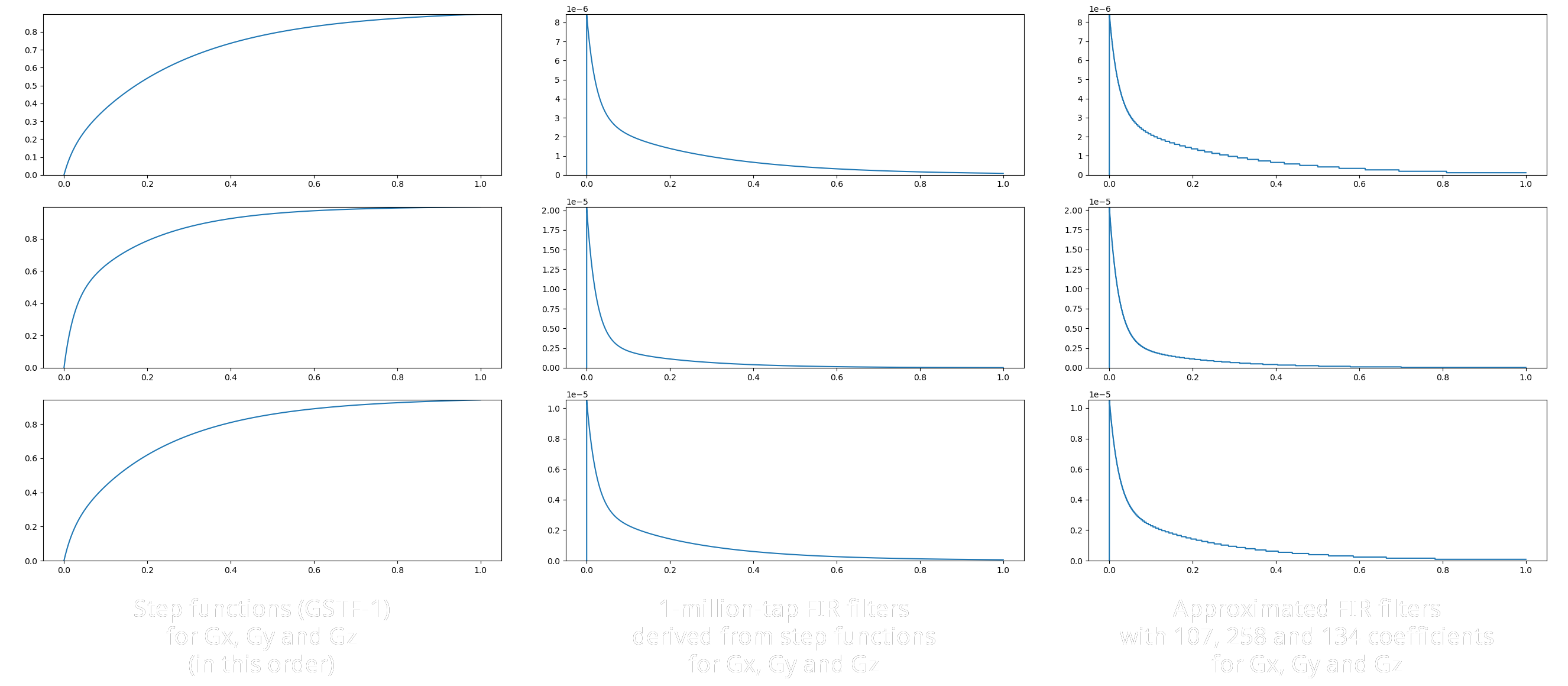
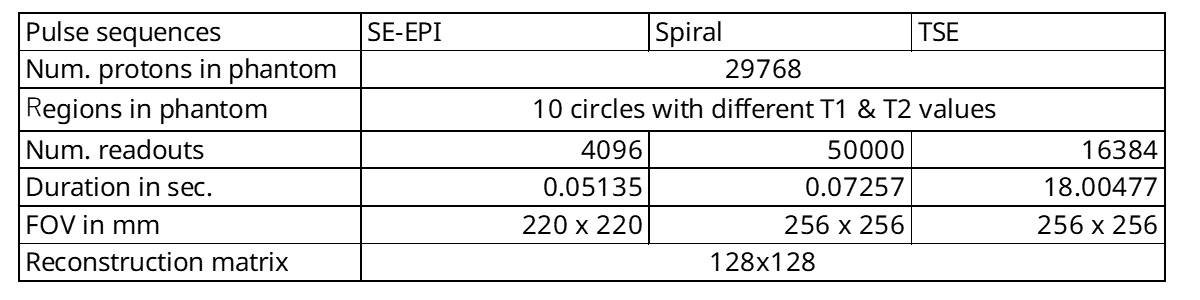
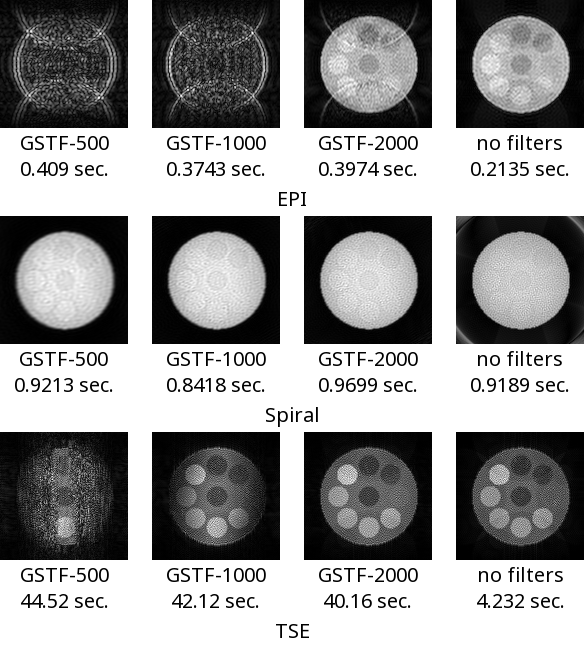
For simulating the GSTF, step response functions GSTF-1, shown in Figure 3, were artificially generated for Gx-to-Gx, Gy-to-Gy and Gz-to-Gz based on the time constants measured in Jehenson et al.³. The functions across coils were not used. To simulate improvements during the past 30 years, step response functions better than GSTF-1 were also generated by dividing time constants by 500, 1000 and 2000 of the original values. These functions were named as GSTF-500, GSTF-1000 and GSTF-2000, respectively. The unit time for processing filters was set to 1 microsecond. The artificial step functions were converted to impulse response functions whose sums over all taps of FIR filters were normalized to 1. The number of taps N was set to a million (corresponding to 1 second). To evaluate the computation time of the proposed method and a standard FIR filter, processing times were measured 10 times by applying them to an ideal step function. The length of the ideal step function was 1 million samples (1 second) for the proposed method and 1 thousand samples (1 millisecond) for the standard FIR filter. The processing times were measured on a 3.6GHz CPU using a Python script with a 64-bit DLL written in C. For demonstrating usefulness of the proposed method, a Bloch simulator was implemented from scratch. The simulator has capabilities to parse pulseq⁶ files and to apply the proposed GSTF to gradients. For all functions of GSTF, single-channel acquisitions were simulated. The acquired data were corrected using the GSTF itself and were reconstructed by a gridding algorithm. The processing times for generating k-space data were measured on the above-mentioned environment. The parameters used in the simulations are given in Figure 4.

Results

The processing times per 1 million samples of the standard FIR filter and the proposed method were $$$2996 \pm 13$$$ seconds and $$$0.970 \pm 0.105$$$ seconds, respectively. The reconstructed images and the processing times for generating k-space data were shown in Figure 5.

Discussion

The experimental results showed that the proposed representation of the GSTF was practical in terms of the computational cost. The results also showed that the proposed method processed GSTF 1000 times faster than a standard FIR filter. Future work will develop models for measuring the GSTF. For the proposed representation, the GSTF should be represented as a function of finite duration. For example, it is possible to use a model based on piecewise functions such as piecewise linear functions and spline curves.

Conclusion

The author proposes a new representation of the GSTF based on FIR filters. The proposed method approximates the GSTF as a piecewise constant function and processes it efficiently using a sliding window algorithm. The experimental results showed that the proposed method could process arbitrary gradient functions in acceptable computational time, without using infinite impulse response (IIR) filters.

References

1. Vannesjo SJ, Haeberlin M, Kasper L, et al. Gradient system characterization by impulse response measurements with a dynamic field camera. Magn Reson Med 2013; 69: 583-593.
2. Stich, M, Wech, T, Slawig, A, et al. Gradient waveform pre-emphasis based on the gradient system transfer function. Magn Reson Med 2018; 80: 1521-1532.
3. Jehenson P, Westphal M, Schuff N. Analytical method for the compensation of eddy-current effects induced by pulsed magnetic field gradients in NMR systems. Journal of Magnetic Resonance 1990; 90 (2): 264-278.
4. Brandenstein H, Unbehauen R. Least-squares approximation of FIR by IIR digital filters. IEEE Transactions on Signal Processing 1998; 46 (1): 21-30.
5. Viola P, Jones M. Rapid object detection using a boosted cascade of simple features. In Proceedings of the 2001 IEEE Computer Society Conference on Computer Vision and Pattern Recognition. 2001. p. 511-518.
6. https://pulseq.github.io/