Introduction

Quality Assurance (QA) is an important part of the MRI studies, ensuring data reliability. Daily phantom scans are part of the manufacturer recommended QA (typically a 5-10 mins EPI stability scan) and weekly, monthly or trimestral phantom scans are usually used by single- or multi-center studies, for control and calibration. Given the sensitivity of spectroscopic imaging acquisitions to B0 and B1 field inhomogeneities, gradient readout imperfections, we propose using a gradient-readout, fast MRSI and a 3D multi-echo GRE acquisition for QA. The metabolite concentrations in a GE manufactured BRAINO phantom, similar to what is typically found in human brain, are 3 to 4 order of magnitude smaller compared to the water signal. While the typical MRSI voxel size is 2 to 3 orders of magnitude bigger, the SNR in a spectroscopy acquisition is still substantially lower than for a regular water imaging acquisition. Thus, stable measurements would indicate normal scanner and coil functioning, while deviations could be detected sooner.

Methods

Gradient readout, fast MRSI acquisition:
Using a 3T Prisma scanner (Siemens, Erlagen, Germany) BRAINO phantom in the centre of either the 32-channel head, 64-channel head or 20-channel head and neck coil, a 30x30x12, 7-mm isotropic rosette spectroscopic imaging (RSI) scan¹ with WET water suppression, TR/TE=1000/19.2ms, FOV=210x210x84 mm3, a 1:48 min:sec water reference (RSI no WET, TR=370ms, FA=15deg), and a 1:28 min:sec 3D GRE scan with same FOV as RSI, 128x128x48 matrix, FA=8, TE1,2,3=2.46/4.92/8.61ms were acquired. Data is reconstructed using rsi_recon (Linux or Windows) and spectroscopic images and spectra are saved to NIFTI and .mat files. When LCModel² is available, siarraysDATA file is processed with lcm_rsi Linux program. Both programs are parallelized, to take advantage of multi-core CPUs. For lcm_rsi, installing Linux “parallels” is recommended, to take advantage of CPU’s hyperthreading, when available. LCModel output for all voxels is read and used to generate baseline-subtracted, 0 and 1st order phased spectra on which SNR for NAA, Cre and Cho is calculated (peak divided to noise standard deviation, calculated in metabolite-free region). Linewidth (LW), metabolite concentrations, CRLBs, LCM SNR, etc are extracted and metabolite concentration and CRLB maps are generated for later visual inspection, if needed. Comma separated (CSV) and Excel files with metabolite concentrations for all voxels, ratios to Cr and CRLBs are generated. Nifti files with spectra and metabolite maps are written out for easy inspection with freeview (part of Freesurfer) or fsleyes (part of FSL). Averages for LW, SNR, etc calculated in central spheroids, around the centre of the acquisition ROI are written to the summary text file. The 3D GRE scan, if acquired, is used to calculate SNR in each coil, as described below for the stand-alone scan and results reported in same summary text file.

Stand-alone multi-echo 3D GRE scan:
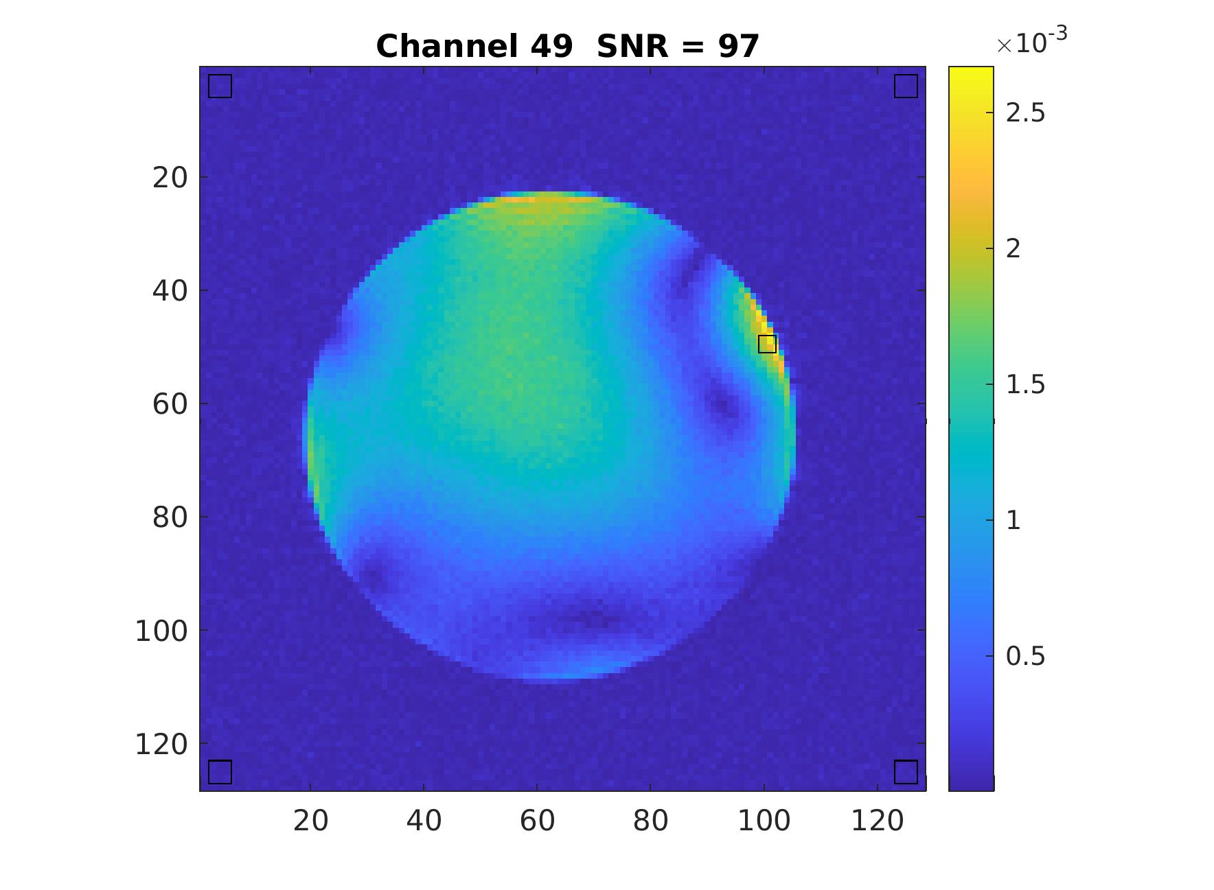
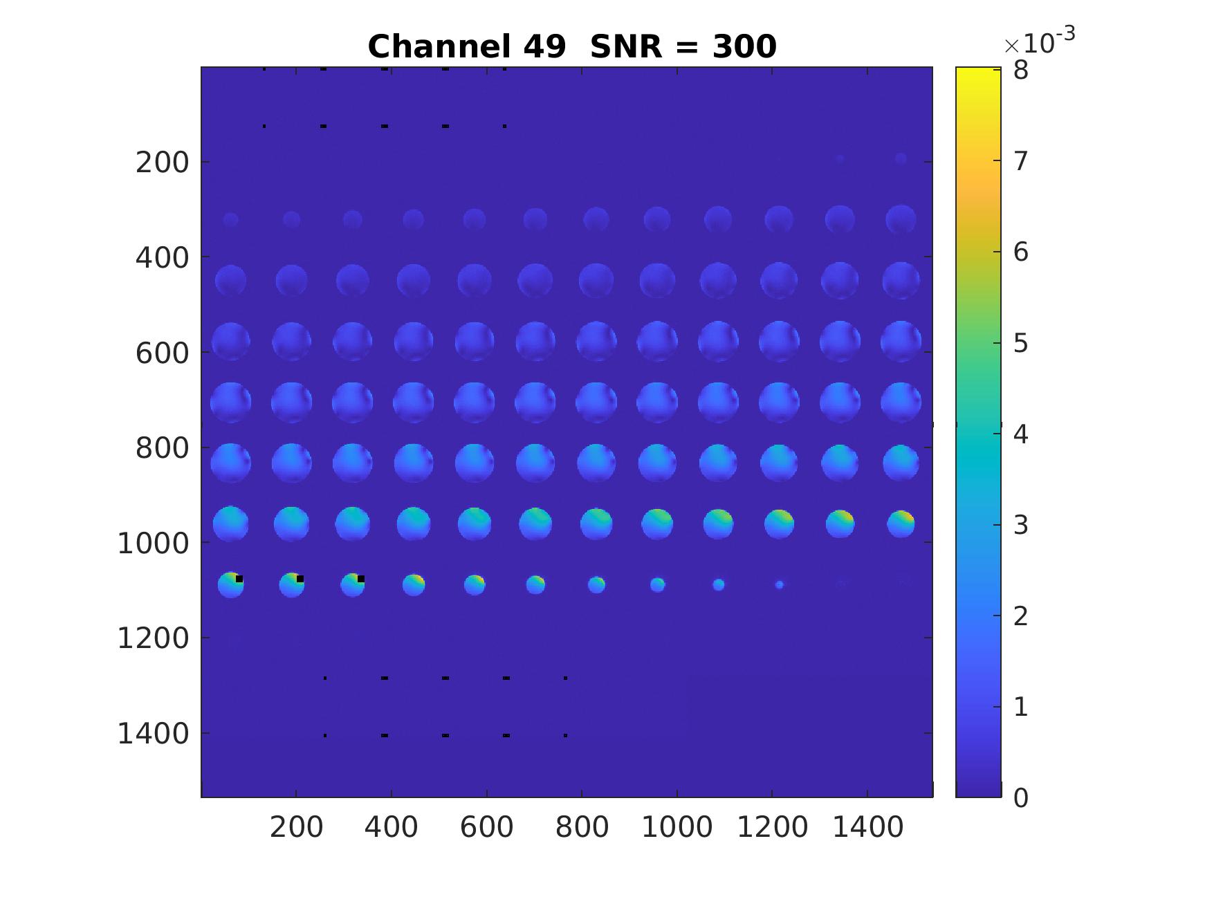
A 3-echo 3D GRE scan as above, but with 128x128x128 matrix and FOV=256mm can be acquired for daily QA. Raw/twix data is reconstructed with greSNR program (github.com/FastMRSI/greQA). SNR is calculated in each channel for the central slice (signal in a square ROI around maximum intensity voxel, noise as standard deviation in square ROIs in the 4 image corners) and an SNR3d is also calculated (signal in a cube ROI around maximum intensity voxel, noise as standard deviation in cube ROIs in the 8 corners). For sum-of-squares combined image signal for SNR is calculated in central square, signal for SNR3d in central cube. The choice of echo times allows for calculation of “water” and “fat” images (even though no fat in phantom we used) as well as B0 maps. While we’ll implement the 3-point Dixon³ for calculations in the future, the water and fat images are currently calculated simply as I2+I3 and I2-I3 with I2 and I3 images corresponding to TE2 and TE3.

Results

Data for one exam and full reconstruction results here: https://pitt.box.com/s/61v6829svyt4lnxapow0st69rtkg6go1
Examples for channel SNR and SNR3d calculations in Figures 1 and 2.

Discussion

We propose using a gradient readout, fast MRSI acquisition for 1-3 months QA and a 3D multi-echo GRE for daily QA. Programs to automatically reconstruct the data and generate simple to read summary text files (in addition to individual coil channels evaluation: SNR, image, etc) are provided (github.com/FastMRSI). In conjunction with a framework such as Yarra (http://yarraframework.com), highly sensitive scanner and coil QA is possible with a high degree of automation.

Acknowledgements

No acknowledgement found.