3333
On the predictability of B0 maps at ultra-high fields using deep learning
Vidya Prasad1, Sharun S Thazhackal1, Ashvin Srinivasan1, Suja Saraswathy1, Jaladhar Neelavalli2, and Umesh Rudrapatna2
1Philips Research, Philips, Bangalore, India, 2Philips Healthcare, Philips, Bangalore, India
1Philips Research, Philips, Bangalore, India, 2Philips Healthcare, Philips, Bangalore, India
Synopsis
UHF-MRI offers increased scanning sensitivity, but suffers from pronounced B0 inhomogeneities. B0 maps are essential for shimming and reconstruction at UHFs, but suffer from scanning overhead and low measurement confidence. Predicting B0 maps from survey scans can effectively address these issues. We assessed predictability of brain B0 maps at 7T and 11.7T using deep learning on a large synthetic B0 map dataset created from 540 CT images. We found that deep learning can predict 1) spherical harmonics for shimming and 2) the complete B0 maps. Our results indicate that B0 predictions work as effectively as acquiring B0 maps for shimming.
Introduction
UHF-MRI shows immense promise for high SNR and high resolution imaging. However, since achieving a good B0 homogeneity is critical for this, higher order shims are commonly used in UHF scanners. Obtaining reliable B0 maps at UHF is crucial as well, as it affects both shimming and also feeds into the reconstruction of many fast scans (EPI, MB-SENSE, spirals etc.). However, acquiring B0 maps consumes time. Moreover, the confidence in the obtained B0 maps typically deteriorates at UHF due to the demands on reducing inter-echo spacing, sometimes leading to phase wraps and thus wrong B0 estimates. The ability to predict B0 maps from structural images (e.g. Survey) can directly reduce the scan time and also potentially provide robust B0 maps.B0 maps depend on anatomical structures that differ across individuals. They also depend on patient positioning, making the prediction challenging. There have been efforts to analytically compute the susceptibility induced B0 inhomogeneity1-4. However, these are computationally expensive and rely on an accurate estimation of the susceptibility distribution, which is challenging due to the indistinguishability of bone and air in MRI. Template-based methods5 overcome these challenges, but their dependency on a database of structural image-B0 pairs, reduces their efficacy with increasing structural variability. Thus, there is a need to develop a more efficient B0 prediction strategy. In this work, we aimed to assess the predictability of UHF B0 maps across a large population using a synthetically generated UHF B0 dataset and deep learning (DL).
Methods
540 head/neck CT datasets were collected from TCIA6-9 and used for learning (Fig. 1). Mastoid, bone, soft-tissue and air were automatically segmented from CT images and susceptibility values of -5.1, -10.3, -9.9 and 0 ppm were respectively assigned. B0 maps were analytically1 computed for field strengths of 7T and 11.7T. These were in turn used as ground truth (GT) for training the DL networks.To generate the learning input, a CT template was first created from 100 randomly sampled CTs, by performing affine and non-rigid co-registration using ANTS10. The voxel-wise mean across the aligned CTs was computed to generate a template. Each CT image was then aligned with the CT template using the same procedure to obtain a composite deformation field (CDF = rotation/stretch/skew + deformation). Since synthetic field inhomogeneity is independent of translations, these were excluded from learning. The CDFs in x,y, and z were used as 3-channel input to the DL network.
Two experiments were conducted. 1) Learning spherical harmonics (image-to-coefficient model): Synthetically generated B0s were decomposed into orthogonal 4th order spherical harmonic (SH) coefficients. The CDFs were resized to 200x200x200. The pairs of CDFs and normalized harmonics were used as input-output pairs to a modified 3D EfficientNet-B011 for training. Weighted-sum-absolute-error loss (with mean batch reduction) was optimized using Adam12. The weights used for SH orders were e0, e-2, e-4, e-7 respectively. 2) Learning B0 maps (image-to-image model): The mean B0 map was computed across all the images and was subtracted from each B0. The respective zero order terms (from brain region) were additionally subtracted from each B0 map. The pairs of the CDFs and B0 maps were re-sized to 128x128x128 and used as input-output to a residual variant of the 3D UNet13. Mean-squared-error loss was optimized using Adam. In both experiments, a random 60-20-20 training-validation-test split was used.
Results
Both the image-to-coefficient model (Fig. 2) and the image-to-image model (Fig. 3) yielded good predictions. The mean absolute errors (MAEs) of the image-to-coefficient model were lower on an average when compared to the image-to-image model, given that the learning problem is simplified by reducing the B0 to 4th order SH coefficients. The models trained on the 11.7T simulations performed slightly better than the predictions at 7T scaled to 11.7T.In order to measure the efficacy of the image-to-coefficient model for shimming, we compared 1) predicted vs GT SH coefficients (Fig. 4) and 2) SD of residuals after shimming using predicted vs GT SH coefficients (Fig. 5). Both the figures show that the image-to-coefficient model is already good enough for shimming.
Discussion
The SD of the residual B0 maps after shimming (Fig. 5) closely matches earlier findings at 7T5,14 and clearly portends the ability to predict UHF B0 maps and shim settings using our proposed approach. The excellent agreement between the predicted and ground truth shim settings (Fig. 4) also corroborates the same. The image-to-coefficient model can be extended to even higher order SH coefficients to capture the GT information more accurately. The image-to-image model also provided good agreement, but can be improved even further with larger datasets, higher resolution learning, better co-registration, hyperparameter optimization etc.Though our work has used CT images, since the success of this approach depends mainly on good co-registration, it can be used with any structural MR image, e.g. Survey and corresponding B0 map. Image co-registration is the only computationally-intensive task in our proposed technique, but we foresee the possibility of sparsifying the input deformation fields significantly through landmarks, which could lead to very fast co-registrations and thus B0 predictions.
Acknowledgements
No acknowledgement found.References
- Koch, Kevin M., et al. "Rapid calculations of susceptibility-induced magnetostatic field perturbations for in vivo magnetic resonance." Physics in Medicine & Biology 51.24 (2006): 6381
- Neelavalli, Jaladhar, et al. "Removing background phase variations in susceptibility‐weighted imaging using a fast, forward‐field calculation." Journal of Magnetic Resonance Imaging: An Official Journal of the International Society for Magnetic Resonance in Medicine 29.4 (2009): 937-948
- Cheng, Yu-Chung N., Jaladhar Neelavalli, and E. Mark Haacke. "Limitations of calculating field distributions and magnetic susceptibilities in MRI using a Fourier based method." Physics in Medicine & Biology 54.5 (2009): 1169.
- Marques, J. P., and R. Bowtell. "Evaluation of a Fourier based method for calculating susceptibility induced magnetic field perturbations." Proc ISMRM. Vol. 11. 2003.
- Shi, Yuhang, et al. "Template‐based field map prediction for rapid whole brain B0 shimming." Magnetic resonance in medicine 80.1 (2018)
- Wee, L., & Dekker, A. (2019). Data from Head-Neck-Radiomics-HN1 [Data set]. The Cancer Imaging Archive. https://doi.org/10.7937/tcia.2019.8kap372n.
- Bejarano T, De Ornelas-Couto M, Mihaylov IB. (2018). Head-and-neck squamous cell carcinoma patients with CT taken during pre-treatment, mid-treatment, and post-treatment Dataset. The Cancer Imaging Archive. https://doi.org/10.7937/K9/TCIA.2018.13upr2xf
- Martin Vallières, Emily Kay-Rivest, Léo Jean Perrin, Xavier Liem, Christophe Furstoss, Nader Khaouam, Phuc Félix Nguyen-Tan, Chang-Shu Wang, Khalil Sultanem. (2017). Data from Head-Neck-PET-CT. The Cancer Imaging Archive. doi: 10.7937/K9/TCIA.2017.8oje5q00
- Grossberg A, Mohamed A, Elhalawani H, Bennett W, Smith K, Nolan T, Chamchod S, Kantor M, Browne T, Hutcheson K, Gunn G, Garden A, Frank S, R osenthal D, Freymann J, Fuller C.(2017). Data from Head and Neck Cancer CT Atlas. The Cancer Imaging Archive. DOI: 10.7937/K9/TCIA.2017.umz8dv6s
- Avants, Brian B., Nick Tustison, and Gang Song. "Advanced normalization tools (ANTS)." Insight j 2.365 (2009): 1-35.
- Tan, Mingxing, and Quoc V. Le. "Efficientnet: Rethinking model scaling for convolutional neural networks." arXiv preprint arXiv:1905.11946 (2019).
- Kingma, Diederik P., and Jimmy Ba. "Adam: A method for stochastic optimization." arXiv preprint arXiv:1412.6980 (2014).
- Ronneberger, Olaf, Philipp Fischer, and Thomas Brox. "U-net: Convolutional networks for biomedical image segmentation." International Conference on Medical image computing and computer-assisted intervention. Springer, Cham, 2015.
- Juchem, Christoph, et al. "Dynamic multi-coil technique (DYNAMITE) shimming for echo-planar imaging of the human brain at 7 Tesla." Neuroimage 105 (2015): 462-472.
Figures
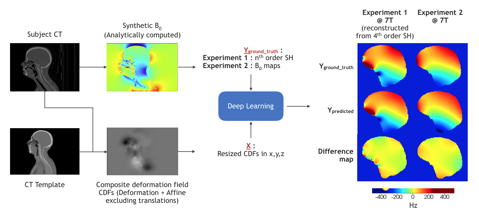
Figure 1. Learning Pipeline Overview : CT images were used to generate synthetic B0 maps via analytical computations1 (Yground_truth). Each CT image was aligned to a template to generate a 3D composite deformation field in x,y,z directions (X). Two experiments were then conducted to predict (Ypredicted) the 1) nth (4th) order orthogonal spherical harmonics using a modified 3D EfficientNet-B011 and 2) whole B0 maps using a residual variant of a 3D UNet13.
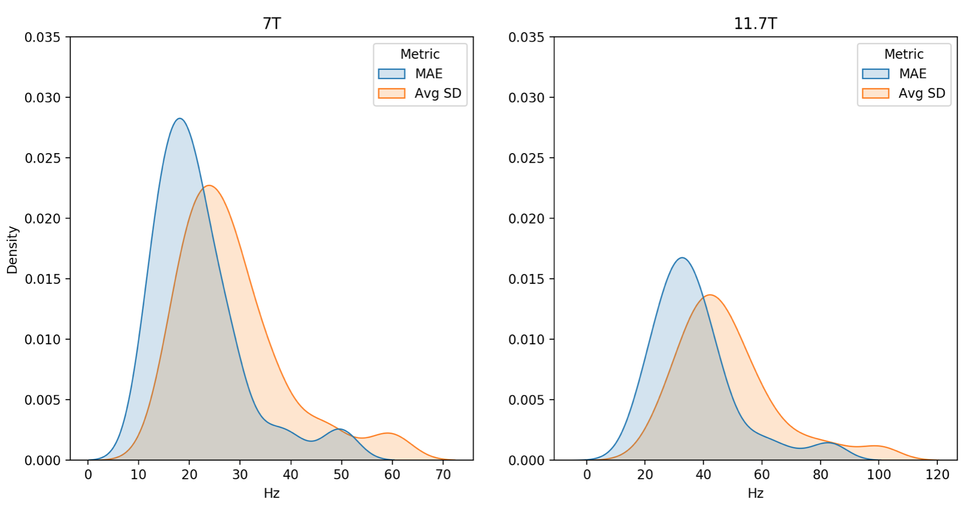
Figure 2. Test performance of image-to-coefficient model. Ground truth and predicted B0 maps were reconstructed using the respective SH coefficients (upto 4th order, excluding 0th term). Reported is the density estimation of the MAE and average standard deviation (Avg SD) across subjects in Hz for each predicted vs ground truth B0 map at 7T (left) and 11.7T (right). Metrics were computed within the brain region only.
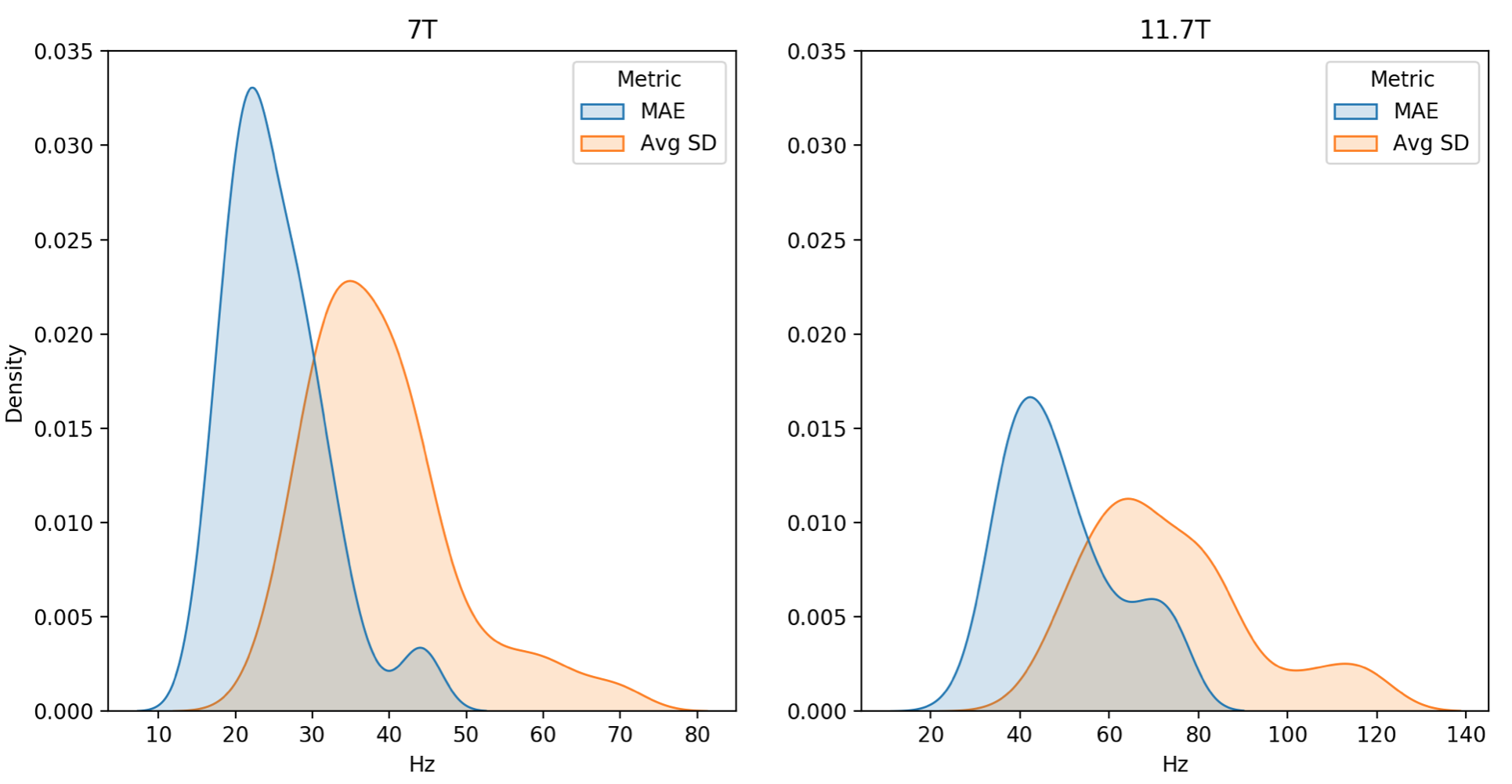
Figure 3. Test performance of the image-to-image model. Reported is the density estimation of the MAE and average standard deviation (Avg SD) across subjects in Hz for each predicted vs ground truth B0 map at 7T (left) and 11.7T (right). Metrics were computed within the brain region only.
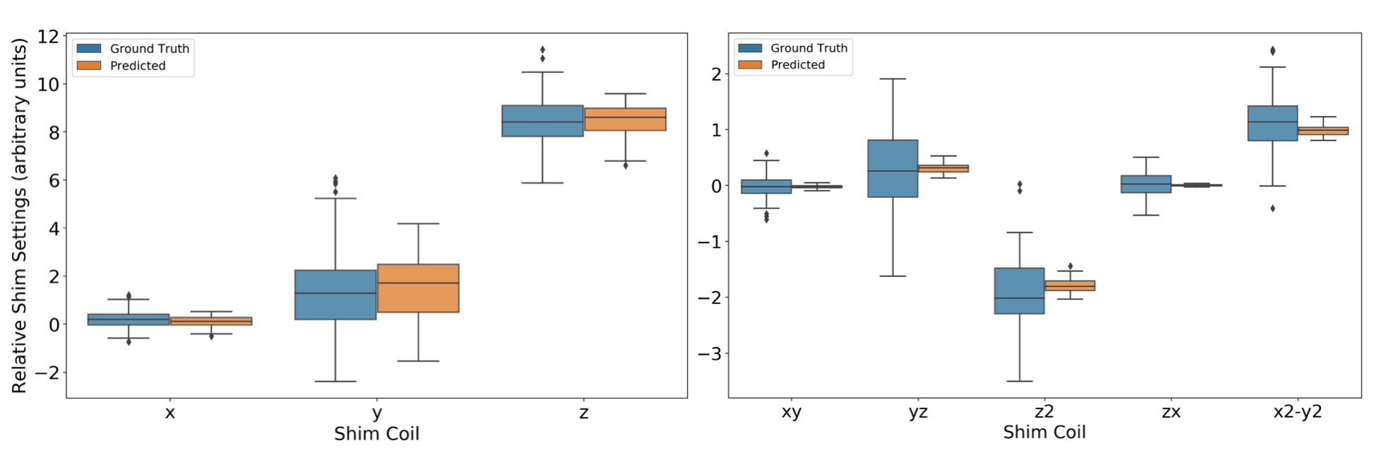
Figure 4. Test set shim predictions of the image-to-coefficient model @ 7T. Reported are the box plots of the predicted and ground truth 1st and 2nd order orthogonal SH coefficients across subjects. The y-axis represents the scaled relative shim values. The x-axis represents each of the 1st and 2nd order shim coils.
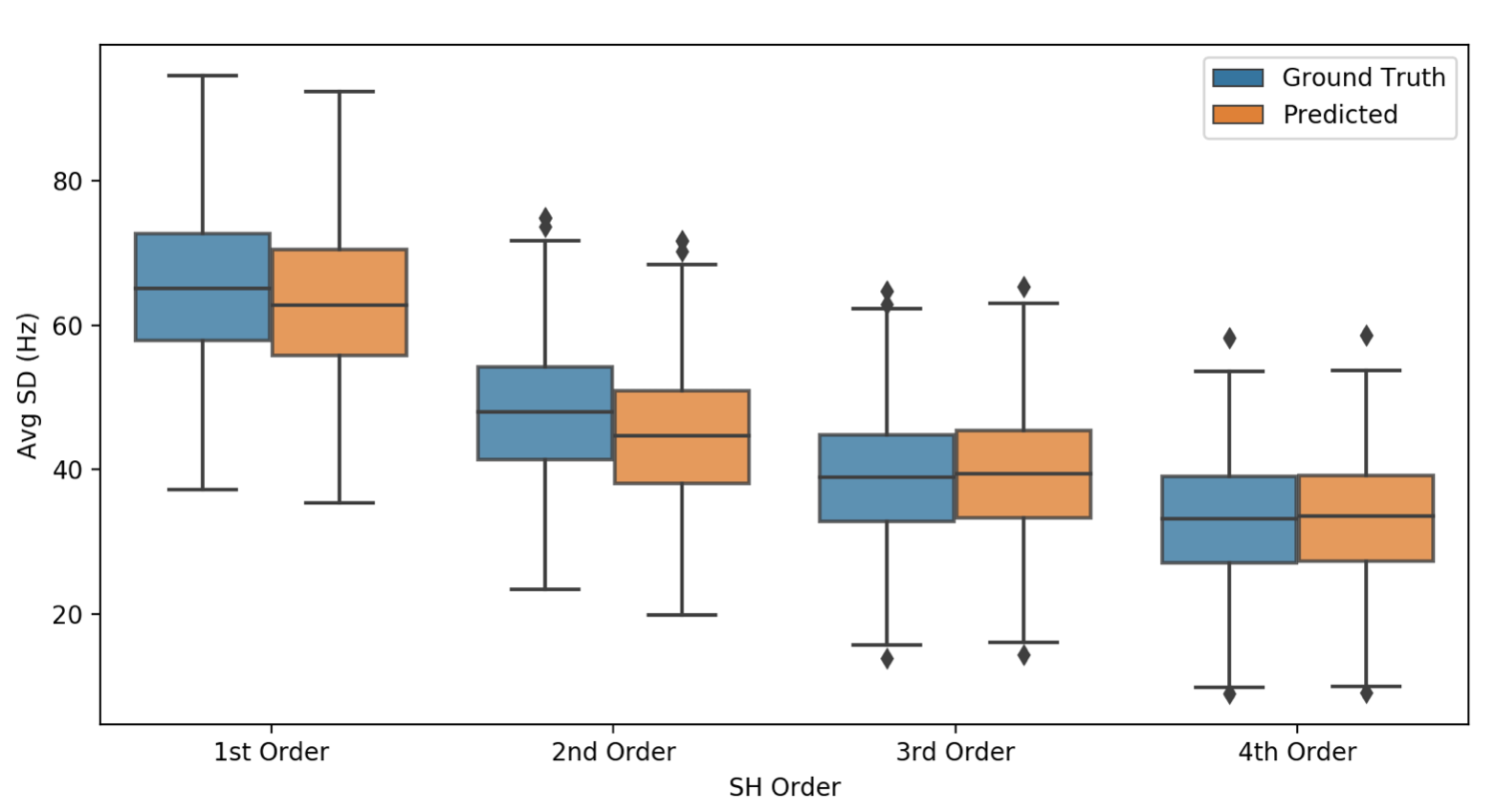
Figure 5. SD of residuals after shimming from image-to-coefficient model @ 7T. Ground truth and predicted B0 maps were reconstructed using upto the 1st, 2nd, 3rd and 4th order SH coefficients (excluding 0th term) respectively. The residuals of the reconstructed maps were computer per order. Reported is the average standard deviation (y-axis) per order (x-axis) in Hz across test set subjects of the predicted and GT residual maps. Metrics were computed within the brain region only.