Introduction

Readout strategies enabling fast k-space sampling such as spiral trajectories are often used in functional and diffusion MRI where ensuring adequate temporal resolution/high data throughput is critical[1]. However, these require fast switching magnetic field gradients, placing high demands on the hardware and compromising output fidelity due, for example, to eddy current fields[2]. These distort the nominal gradient time-courses impacting the traversed k-space trajectory[3]. It is possible to reduce image artefacts, by taking into account, during reconstruction, the effective gradients. Using linear systems theory, the net response can be modeled as a gradient impulse response function (GIRF)[4].
We present an open-source calibration of the GIRF for gradient characterization to account for delays and induced eddy-currents. For illustrative purposes, we focus on application to spiral readouts, presenting simulations and preliminary phantom results.

Methods

We considered three steps: firstly, we implemented a pulse sequence to measure the system GIRF using the open-source tool PyPulseq[5]; secondly, to demonstrate its impact in reconstruction, we did a simulation study using spiral gradient trajectories distorted by the measured GIRFs; finally, the GIRF measurement and spiral readout correction were tested on a real scan.
The gradient system response is characterized by the GIRF h(t), relating the input i(t) and the obtained output, o(t) [6]:

$$$ o(t) = \int_{-\infty}^{\infty} i(\tau) \cdot h(t-\tau) d\tau \leftrightarrow (FT) \leftrightarrow O(\omega)=I(\omega) \cdot H(\omega) $$$ (1)

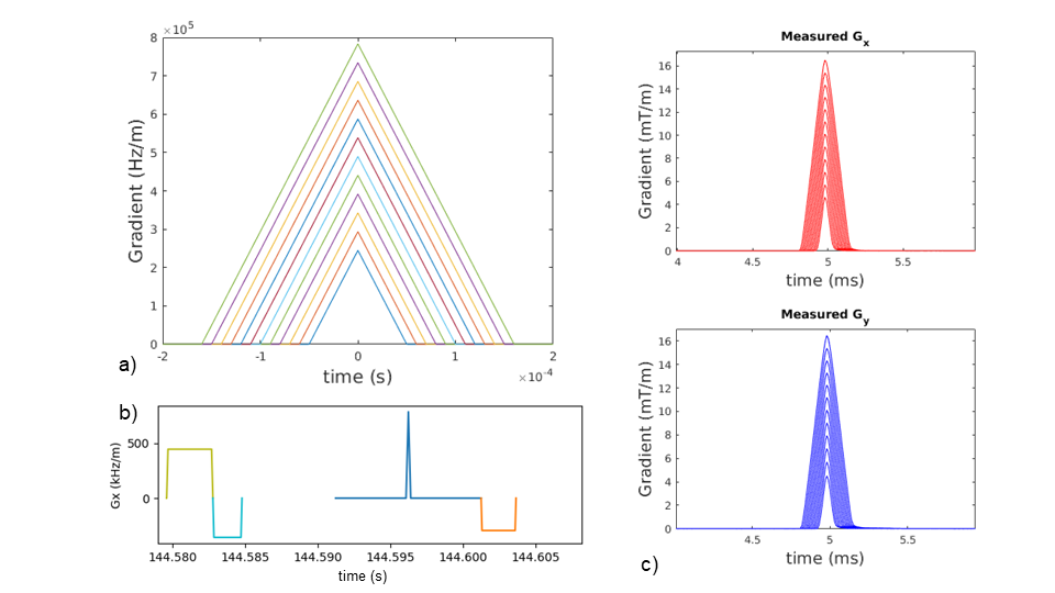
where t and denote time and angular frequency, and O(W), I(W) and H(W) represent the Fourier transforms (FT). It is possible to estimate the GIRF using triangular gradient pulses to sample different frequency ranges, and measure the effectively produced gradients[4]. To estimate the GIRF - H(W), we adapted the work[2] by measuring the produced gradient waveforms using the Duyn approach (Figure 1), which does not require additional hardware (i.e. field monitoring probes), unavailable at most sites. The sequence was implemented in Matlab®, using the original PyPulseq, and Python®. The triangular pulses and sequence parameters are described in Figure 1. To estimate the GIRF from the data, code implemented in[7] was used.
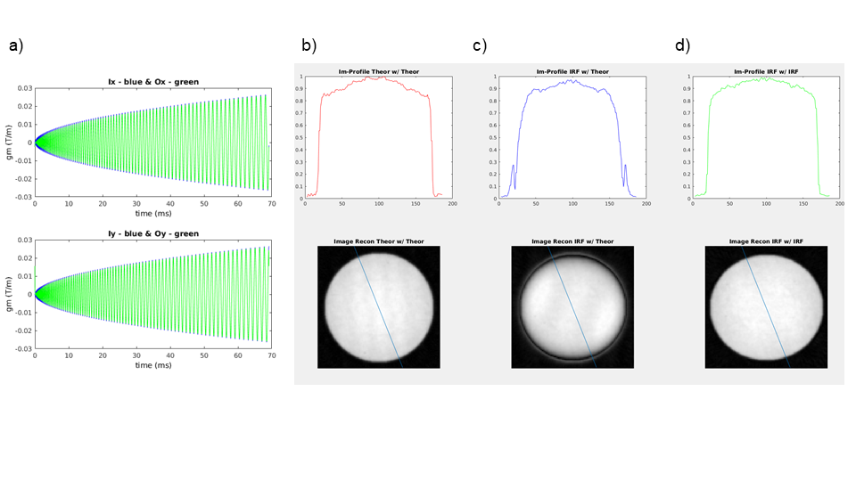
Simulations were performed using JEMRIS [8]. To evaluate the impact of the GIRF on the reconstructed images, avoiding confounding effects (e.g. B0 inhomogeneities), three tests were made for the same spiral sequence: a) simulating data acquisition and performing reconstruction using nominal gradient waveforms (Theo-Theo), b) simulating the impact of the measured x- and y-axis GIRFs on the waveforms but using the nominal trajectory in reconstruction (GIRF-Theo) and c) considering the measured scan GIRFs in the acquisition and reconstruction (GIRF-GIRF). A spherical sample was considered (Figure 1), and image profiles compared between tests. Images were reconstructed using the Gridding tool (https://github.com/wandell/mrTutorials-matlab) (kernel_width=3, with Voronoi density compensation), followed by Fast FT.
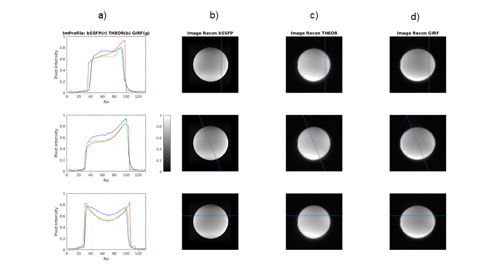
The same spiral sequence was used to image a phantom in a Siemens Aera 1.5T scanner. A balanced steady state free precession (bSSFP) readout, less susceptible to geometric distortions, was used as reference (TR/TE=3.04/1.52 ms, FA=35º, 6mm slice thickness, field-of-view 200×200 mm2, and 128×128 matrix). Data was reconstructed offline in MATLAB. The spiral data was reconstructed both with and without considering the measured GIRFs. Images were compared visually and evaluated using an edge-sharpness (ES) metric - distance between the 20%-80% of maximum profile amplitude[9].
All the code is available at https://github.com/ZemaTimoteo/GIRFOS_tool.

Results

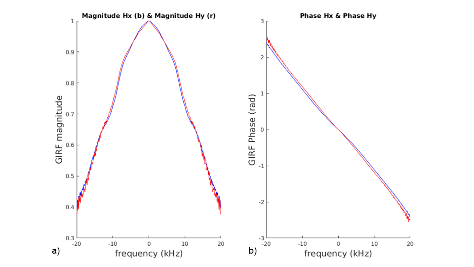
The measured GIRF magnitude and phase are depicted in Figure 2, exhibiting low-pass characteristics as expected. The simulations (Figure 3) suggest that by considering the effective k-space trajectory, a more faithful object representation is obtained as b) and d) are more alike. When the nominal spiral trajectory is used to reconstruct data simulated with GIRF-distorted gradients, ripples can be seen near image edges.
The scanner results (Figure 4) confirm that the GIRF-corrected spiral mitigates eddy-current effects, with d) closer to b) than c). The depicted image profile shows that although the bSSFP image is the sharpest (mean ES over the three slices: 4.5mm), the corrected spiral image (mean ES=6.5mm) is less blurred compared to when using the nominal spiral trajectory (mean ES=8.3mm).

Discussion

Using the GIRF to predict the executed gradient waveforms mitigates the impact of the induced eddy-currents enabling to improve the reconstructed image[4]. Using the method proposed in[2], provided a plausible estimate for the GIRF. Although the GIRF-corrected reconstructed images were shown to more closely follow the bSSFP geometry, further improvements should be attainable as other sources of artifacts were not considered. Future work will target B0 eddy-current effects[10] and blurring induced by off-resonance[3].
This work was developed within the Open-Source imaging initiative (https://www.opensourceimaging.org/), aiming to improve accessibility to MRI. By providing an open tool for calibrating MRI system’s GIRF, we hope to contribute towards attaining good quality open-source images using less stringent hardware requirements, reducing costs and helping to make MRI available to a wider population.

Conclusion

This work demonstrated the use of a GIRF calibration method based on an open-source sequence implemented using Pypulseq. As well as illustrating the impact of the measured GIRFs through simulations, improvements in real phantom images were demonstrated when considering the GIRF measurements in the reconstruction. The implemented pipeline provides a fast and easy gradient system characterization, helping to account for linear distortions, as produced by eddy-current fields, resulting in improved image quality.

Acknowledgements

This work was supported by Fundação para a Ciência e a Tecnologia (FCT) - (grants PTDC/EMD-EMD/29686/2017, UID/EEA/50009/2019 and UIDB/50009/2020) and Programa Operacional Regional de Lisboa 2020 (LISBOA-01-0145-FEDER-029686).