Introduction

One of the many challenges of ultrahigh field strengths In MRI is inhomogeneity of B0 field. In clinical MRI system shimming hardware is available till either first order or till the second order. For the high field systems inhomogeneity of B0 field creates various artifacts. Vendor implemented B0 shimming algorithm assumes that the shim fields generated by each coil are identical to the desired spherical harmonic function. If this is not the case, then to improve shim shimming needs to be done iteratively. The alternate approach is to acquired field maps and for each shim coil to correct field inhomogeneity [1].

Methods

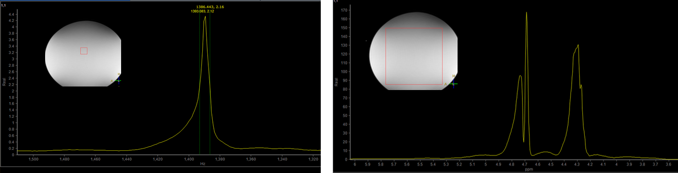
All data was acquired at a Philips Achieva 7T whole body human MR imaging system (Philips Healthcare, Amsterdam, Netherlands) with a dual TX head coil (Nova Medical). The vendor implemented B0 shim system consists of one 0th order, three 1st order, five 2nd order and seven 3rd order shim coils.
To investigate the quality of the vendor implemented shim system calibration matrix non-water suppressed spectra using a PRESS sequence were acquired from a small voxel in the isocenter (20x20x20 mm) and a large voxel (200x200x200 mm) encompassing large parts of a spherical phantom. The phantom had a diameter of 300 mm and contains 0.011g MACROLEX blue per liter.

To further characterize the shim system reference field maps of each shim coil were measured using the same spherical phantom. The B0-mapping sequences had a delta TE of 0.25ms, as this ensures that fat and water are in phase, and it minimizes the amount of phase wrapping in the B0 map. Any phase unwrapping that was required was performed using FSL prior to further analysis. The reference fields of each of the 15 shim coils were acquired at a different range of current amplitudes in order to determine the relationship between shim field strength and output current strength of the shim amplifier, which also varies for each shim coil [1].

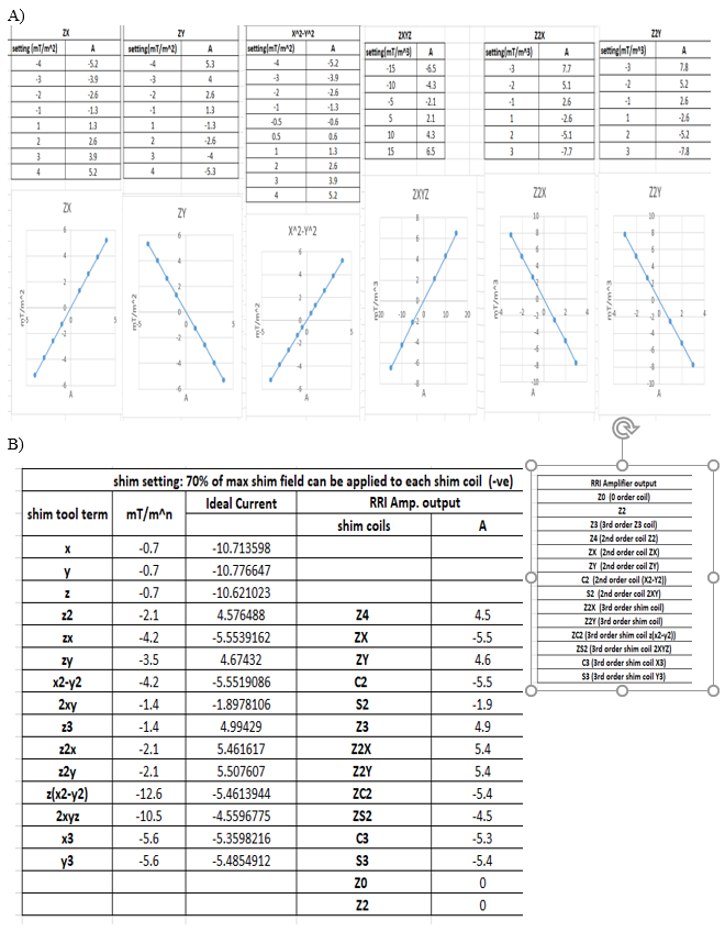
To further investigate the linearity of the shim amplifiers each shim coil was first selected individually, and the respective relationship between the respective shim field (in mT/mn) and the applied current (in A) was measured from the shim amplifier (Resonance Research Inc). In addition, all shim amplifier modules for all shim coils were operated at ones in another test.

Results & Discussions

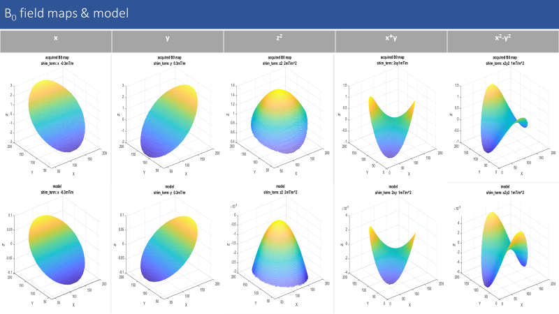
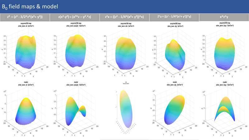
Figure 1 (a) shows the non-water suppressed spectra for a small voxel (20x20x20 mm) in the isocenter and a large voxel (200x200x200) mm in a spherical phantom (per Liter MARCOL-oil: 0.011g MACROLEX blue). While the vendor pre-implemented 3rd order shimming routine converges in the small voxel; this is not the case for the large voxel. Hence the shim calibration done by vendor’s implemented method is not suitable for the large voxel 3rd order B0 shimming.

A comprehensive characterization was performed to investigate further. Figure 2 and 3 show the acquired field maps of different shim terms and the ideal shim field models representing spherical harmonic functions. The upper row in both figures shows the acquired field maps for different shim fields and the bottom row shows the respective ideal shim field models . We can clearly see that for the first order and second order shim coils the acquired field maps and ideal shim field models are almost identical for all respective shim terms. But for the third order shim terms there is a strong linear term present in all the acquired real field maps for all shim terms and there is not much difference in between the acquired field maps for different third order shim coils. This finding demonstrates the need for real shim calibration and the limitation of the 3rd order shim system at hand due to a lack of orthogonality of it’s shim terms.

Figure 4 (a) shows the linear behavior of shim amps. When we turn on each shim coil individually and apply shim field gradually the change in current with respect to applied shim field is linear. In Table 1 (b) we have applied 70% of maximum shim field applicable for all shim coils and still confirm a linear behavior and a close match of measured and theoretical shim field and shim current values.

In future work the full shim calibration matrix will be derived from these data and implemented into a custom written shim software. Instead of using Vendor's implemented algorithms, we will use the acquired real shim field maps and model these real shim fields as a linear combination of ideal spherical harmonic shim fields of different orders [1].

Conclusion

The vendor implemented 3rd order shim system of a 7T whole-body human MRI scanner was characterized. It was found that the shim system shows a linear behavior of the relationship between shim current strength and shim field strength. The 1st and 2nd order spherical harmonic shim coils produce shim fields that closely match the ideal shim fields. However the 3rd order spherical harmonic shim coils produce shim fields that largely deviate from the ideal shim fields and exhibit strong linear field contaminations. This demonstrates that successful 3rd shimming requires a real shim field calibration and a shim system that delivers orthogonal 3rd order shim terms.

Acknowledgements

This work was performed at the facilities of Advance Imaging Research Center (AIRC) at the University of Texas Southwestern Medical Center from Cancer Prevention and Research Institute of Texas (CPRIT) grant / RR180056.