Introduction

Fat-water ambiguity is an intrinsic problem from chemical shift encoded imaging model¹. When this problem is not well solved throughout the whole image, fat-water swaps appear and result in inaccurate fat quantification. The success of solving the ambiguity relies on pre-assumptions, e.g. the magnetic field continuity^{1, 2} or the prior knowledge of the adipose/aqueous tissue distribution³ etc. In our work, we proposed to incorporate the T1 difference of fat and water to help solve the ambiguity problem.

Theory

Generally fat has shorter T1 than water in most tissues. Chemical shift encoding is mostly based on multiple echo gradient echo (GRE) sequence with short TR, and water fat signal ratio is flip angle (FA) dependent due to T1 difference.
Fat-water ambiguity
Three echoes were acquired under each FA. Signal model for evenly spaced echo times $$$[TE_{2}-\Delta TE,TE_{2},TE_{2}+\Delta TE]$$$ is:
$$$S_{1}=(W+F\cdot {e^{-i2\pi f_{F}(TE_{2}-\Delta TE)}})e^{-i2\pi\Psi(TE_{2}-\Delta TE)}$$$
$$$S_{2}=(W+F\cdot^{-i2\pi f_{F}TE_{{2}}})e^{-i2\pi \Psi TE_{2}}$$$
$$$S_{3}=(W+F\cdot {e^{-i2\pi f_{F}(TE_{2}+\Delta TE)}})e^{-i2\pi\Psi(TE_{2}+\Delta TE)}$$$ (1)
W and F are signal intensities; $$$\Psi$$$ is field inhomogeneity.
Let $$$\widetilde{W}=W\cdot e^{-i2\pi \Psi TE_{2}}$$$, $$$\widetilde{F}=F\cdot e^{-i2\pi \Psi TE_{2}}\cdot e^{-i2\pi f_{F} TE_{2}}$$$, we have:
$$$S_{1}=(\widetilde{W}+\widetilde{F}\cdot {e^{-i2\pi f_{F}(-\Delta TE)}})e^{-i2\pi\Psi(-\Delta TE)}$$$
$$$S_{2}=\widetilde{W}+\widetilde{F}$$$
$$$S_{3}=(\widetilde{W}+\widetilde{F}\cdot {e^{-i2\pi f_{F}(\Delta TE)}})e^{-i2\pi\Psi(\Delta TE)}$$$ (2)
Suppose $$$\Psi _{t}$$$ is true solution, corresponding aliased solution was given by¹:
$$$\Psi _{a}=\Psi _{t}+\frac{arg(\frac{\widetilde{W}+\widetilde{F}\cdot e^{i2\pi f_{F}\Delta TE}}{\widetilde{F}+\widetilde{W}\cdot e^{i2\pi f_{F}\Delta TE}})}{2\pi \Delta TE}=\Psi _{t}+\frac{1}{2\pi \Delta TE}\cdot {arg[({W+F\cdot e^{-i2\pi f_{F}TE_{2}}\cdot e^{i2\pi f_{F}\Delta TE}})/({F\cdot e^{-i2\pi f_{F}TE_{2}}+W\cdot e^{i2\pi f_{F}\Delta TE}}})]$$$ (3)
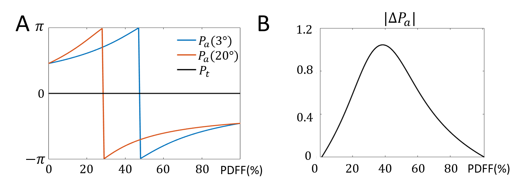
$$$\Psi _{a}$$$ is also solution to Equation 1, but resulting in swapped fat-water components. $$$\Psi _{t}$$$ should be almost the same under different FA, while aliased solution should be different according to Equation 3. To avoid phase wrapping, phase factor (or phasor)⁴ was introduced as $$$P=e^{i2\pi \Psi \Delta TE}$$$ in following parts. $$$P_{t}$$$ and $$$P_{a}$$$ are true and aliased phasor solution, and FA dependency can be expressed as:
$$$P_{t}(\theta_{1})=P_{t}(\theta_{2})$$$
$$$P_{a}(\theta_{1})\neq P_{a}(\theta_{2})$$$ (4)
Defining
$$$\Delta P_{a}=abs(angle(P_{a}(\theta _{1})*conj(P_{a}(\theta _{2}))))$$$ (5)
as the differences of aliased phasor solution under two FAs, $$$\Delta P_{a}$$$ is non-zero when PDFF≠0% or 100%, as in Figure 1.
Fat-water separation
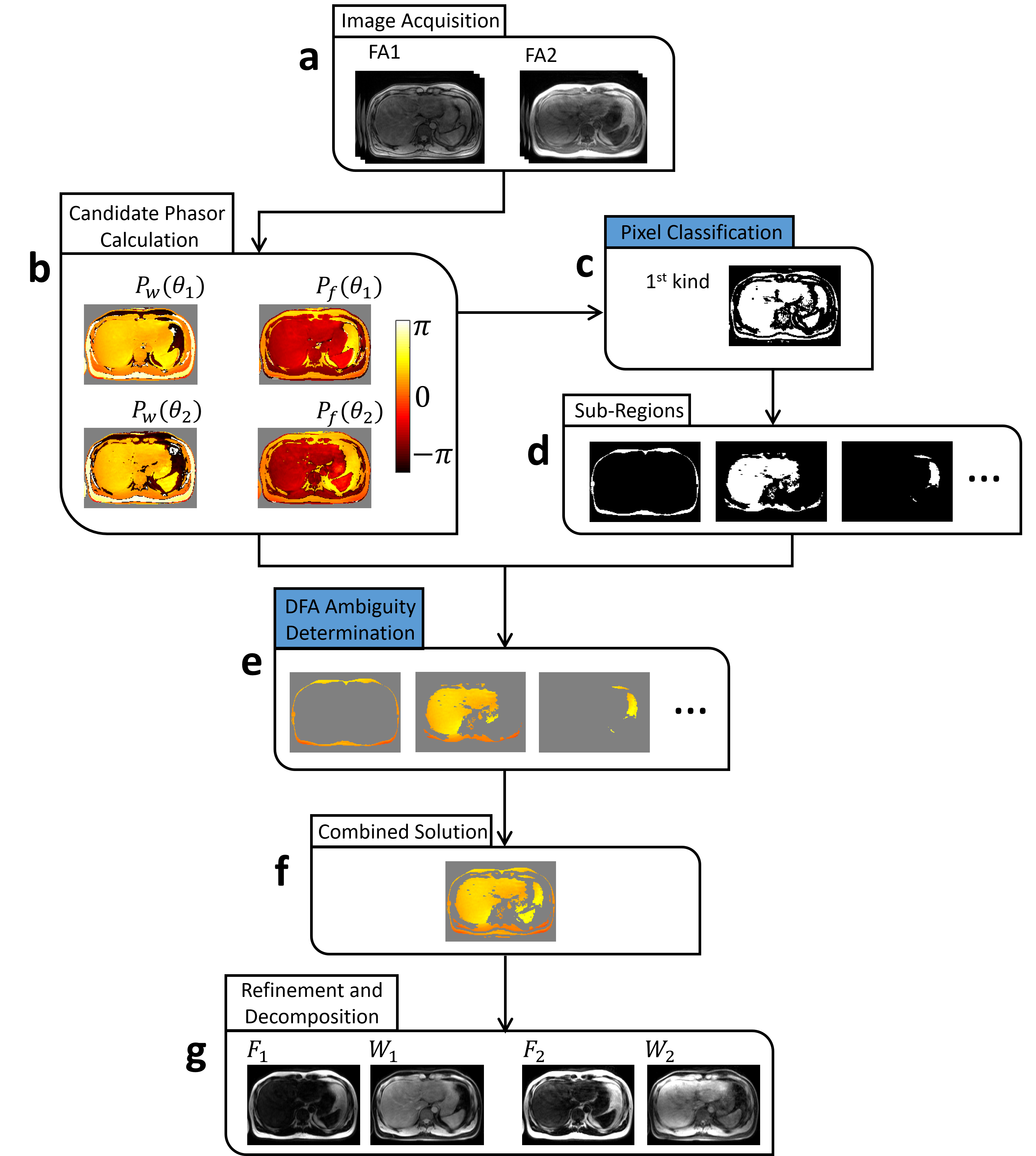
The flowchart of proposed method was shown in Figure 2. The algorithm is introduced step by step.
Candidate phasor solutions were calculated as ref⁵. Phasor solutions was classified into two groups $$$P_{w}$$$ and $$$P_{f}$$$, corresponding to water and fat-dominant results respectively⁶, as Figure 2b.
All pixels were classified to two kinds. First, pixels with their phasor solutions similar to those of all 6-neighbors in 3D were defined as “smooth” pixels; Second, the left pixels were defined as “non-smooth” pixels. Define $$$D_{w}(r)$$$ as the maximum phasor difference in $$$P_{w}$$$ between pixel r and its neighborhood $$$r_{k}$$$:
$$$D_{w}(r)=max_{k}|angle[P_{w}(r)\cdot conj(P_{w}(r_{k}))]|$$$ (6)
k denotes the index of 6-neighborhood pixels in 3D direction. $$$\left | \cdot \right |$$$ is absolute operator. $$$D_{f}(r)$$$ is defined in the same way. When all of the $$$D_{w}(r)$$$ and $$$D_{f}(r)$$$ under different FAs are smaller than threshold $$$D_{T}$$$, the pixel r is considered as ”smooth pixels”. The mask of the “smooth” pixels was shown in Figure 2c.
The “smooth” pixels were grouped to sub-regions according to spatial connectivity, as shown in Figure 2d. According to definition of “smooth” pixels, spatially connected “smooth” pixels have similar solutions, and true solutions must belong to same category (either $$$P_{w}$$$ or $$$P_{f}$$$). Consequently, the solution determination of a single sub-region was transformed into a binary choice.
The FA-dependencies of $$$P_{t}$$$ and $$$P_{a}$$$ are exploited to determine the true solutions for each sub-region. Specifically, when
$$$\sum _{r\in \Theta_{j}}|P_{w}(r,\theta_{1})-P_{w}(r,\theta_{2})|< \sum _{r\in \Theta_{j}}|P_{f}(r,\theta_{1})-P_{f}(r,\theta_{2})|$$$ (7)
where $$$\Theta_{j}$$$ denotes all pixels in the j-th sub-region, the true solutions in $$$\Theta_{j}$$$ are chosen as:
$$$P_{t}(r)=P_{w}(r),r\in \Theta_{j}$$$ (8)
and vice versa.
After determination of each sub-region, phasor solution was combined together, as in Figure 2f. Solutions of residual pixels was determined by region growing scheme, with consideration of six-peak fat spectral model and $$$T_{2}^{\ast }$$$ decay.

Materials and Methods

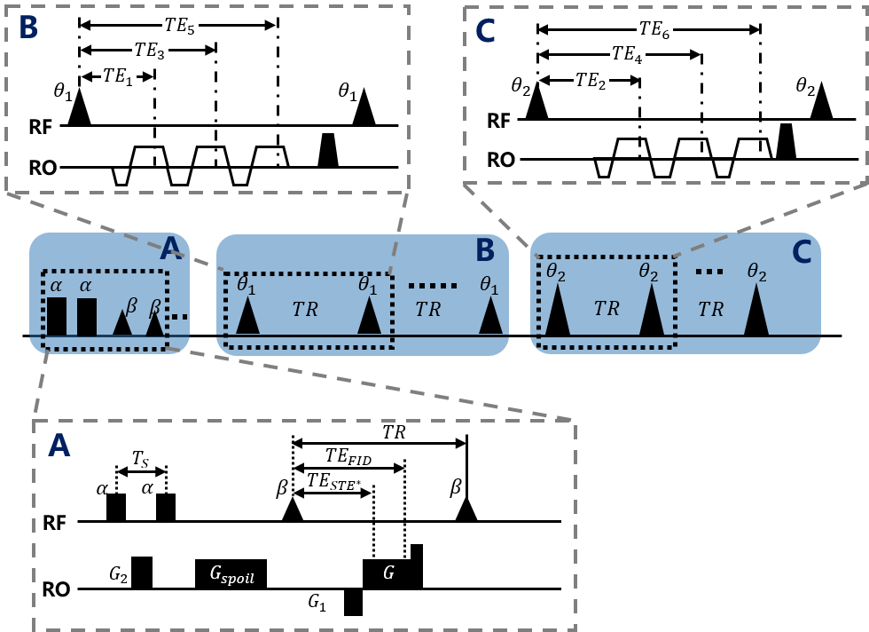
Six echo acquisition was divided into two three-echo acquisition with different FAs. The pulse sequence is depicted in Figure. 3. Optionally, a B1+ mapping sequence based on DREAM⁷ was incorporated if accurate T1 mapping was desired.
Two volunteers were recruited with informed consent under IRB approval, imaging parameters of the GRE images for both volunteers were: FOV=240*400*160 mm³, resolution=1.92*1.92*4 mm³, bandwidth = 1300Hz/pixel, TR = 6.7ms, flip angle = , TE1/3/5 = 1.42/2.86/4.3ms for FA=3°, and TE2/4/6 = 2.14/3.58/5.02ms for FA=20°. The scan was finished in a single breath-hold with Parallel imaging and partial Fourier acquisition, total acquisition time = 16.3s. Parameters for fat-water phantom were omitted for simplicity, using TREE⁶ and IR-FSE⁸ as reference.

Results

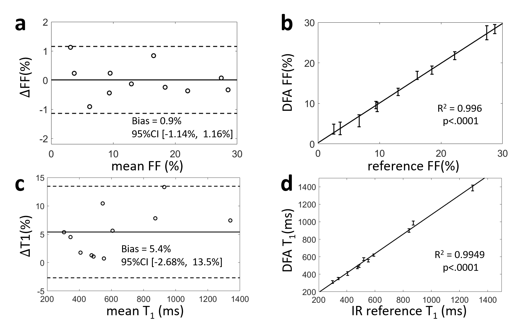
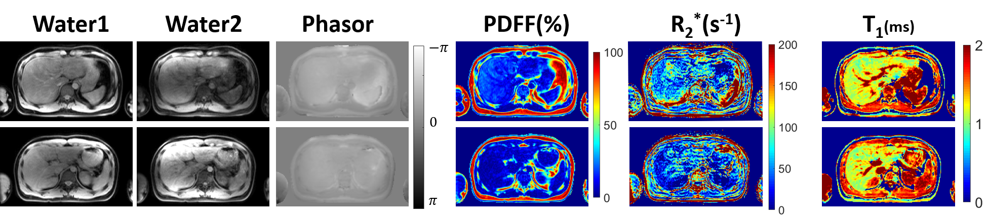
Proposed method separated fat and water signals in both phantom and volunteer studies. The resultant PDFF and T1 values showed high consistency to reference values, as shown in Figure 4. Simultaneous T1/PDFF/R₂* quantification were realized within a single breath-hold by the proposed method, as shown in Figure 5.

Discussion and conclusions

A fat-water separation algorithm based on dual flip angle acquisition was designed in this work. Under dual flip angle, the T1 difference between fat and water can serve as a new priori information in solving fat-water ambiguity. Moreover, the proposed method can obtain PDFF and accurate T1 mapping simultaneously with B1+ correction. The sequence could cover the whole liver within a single breath-hold.

Acknowledgements

No acknowledgement found.