3292
Why You Should Fit Signal Intensity, Not Relaxivity, for Quantitative DCE-MRI1Oden Institute for Computational Engineering and Sciences, The University of Texas at Austin, Austin, TX, United States, 2Livestrong Cancer Institutes, The University of Texas at Austin, Austin, TX, United States, 3Department of Radiology, University of Washington, Seattle, WA, United States, 4Department of Biomedical Engineering, The University of Texas at Austin, Austin, TX, United States, 5Department of Diagnostic Medicine, The University of Texas at Austin, Austin, TX, United States, 6Department of Oncology, The University of Texas at Austin, Austin, TX, United States
Synopsis
Pharmacokinetic modeling of DCE-MRI is based on fitting perfusion parameters to contrast agent concentration or relaxivity curves computed using the nonlinear spoiled gradient-echo (SPGR) signal equation, T1 mapping values, and the linear relationship between T1 and contrast agent relaxivity. The nonlinear term of the SPGR equation has implications for how image noise scales in the concentration. By simulating image noise at different levels for ideal curves of different parameter values, we show why it’s advantageous to fit signal intensity curves rather than relaxivity curves.
Introduction:
Dynamic contrast-enhanced MRI (DCE-MRI) is used qualitatively to identify tumors for cancer diagnostics since after administering a contrast agent, suspicious lesions significantly brighten with respect to surrounding healthy tissue due to a combination of greater delivery and retention. However, when one seeks to quantify this change, DCE-MRI with high temporal resolution must be used to obtain time course data for pharmacokinetic (PK) modeling of (for example) blood flow, vessel permeability, and tissue volume fractions [1,2]. These measures have shown success in predicting therapy outcome from longitudinally-acquired exams acquired before and during treatment [3,4].For estimation of PK parameters, two key measurements are required: 1) a pre-contrast map of the native T1 (T10) of tissue, and 2) heavily T1-weighted images rapidly acquired before, during, and after the injection of the contrast agent. These two data, along with the repetition time and flip angle, are then used with the spoiled gradient echo signal equation to convert the signal intensity time series to a relaxivity time series. By assuming fast water exchange and knowing the relaxivity of the contrast agent used, the linear relationship between tissue relaxivity and contrast agent concentration provides a time course of contrast agent concentration in each voxel. Finally, the time-varying tissue contrast concentration and an assumed (or measured) post-injection blood plasma concentration (i.e., the arterial input function) is used with the Kety-Tofts (or another) PK model to estimate the volume transfer constant (Ktrans) and extracellular volume fraction (ve).
The non-linearity of the exponential relaxivity term in the SPGR equation leads us to expect that any image noise will be amplified for images when contrast agent concentration peaks, leading to greater error in estimated parameters. In this work we simulate parametric curves with varying noise levels to systematically determine whether standard Kety-Tofts fits are more accurate when the model is fit to the signal intensity time course instead of the relaxivity or contrast agent concentration time course, and we present an example from images acquired and compared in a breast cancer study.
Methods:
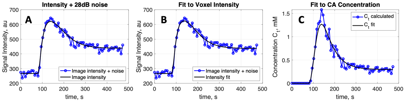
A range of Kety-Tofts standard model parameters Ktrans and ve were selected to compute a set of noiseless concentration (Ct) and signal intensity (SI) curves. A family of simulated data was constructed by adding Gaussian noise at a range of signal to noise levels (SNRs) to the signal intensity curves . The experiment of adding noise to each SI curve was repeated 1000 times for each simulated noise level. For each combination of parameters and noise levels, standard Kety-Tofts perfusion models were fit to both the simulated noisy signal intensity curves, and the contrast agent concentration curves computed from the simulated noisy signal intensity curves. Estimated Ktrans and ve values returned from both sets of fits were compared to determine average errors. Figure 1 shows one example of the simulated noisy curves and Ktrans fits. Vectors of the differences between simulated Ktrans parameters and each of the fit resulting Ktrans (fitting signal intensity and fitting concentration) were compared using a paired t-test at the 5% significance level. Finally, standard Kety-Tofts parameter maps were created from model fits to signal intensity and concentration curves in DCE-MRI data from 22 breast cancer patients that were scanned with IRB approval and informed consent given as part of an ongoing treatment response monitoring study. Alongside the maps for comparison, estimated noise maps from the fit residuals were compared visually.Results:
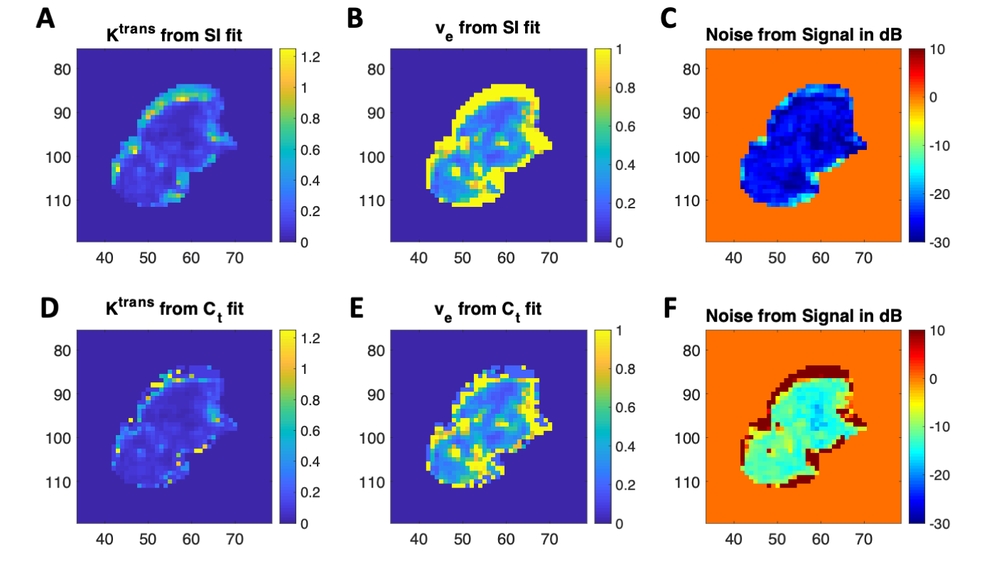
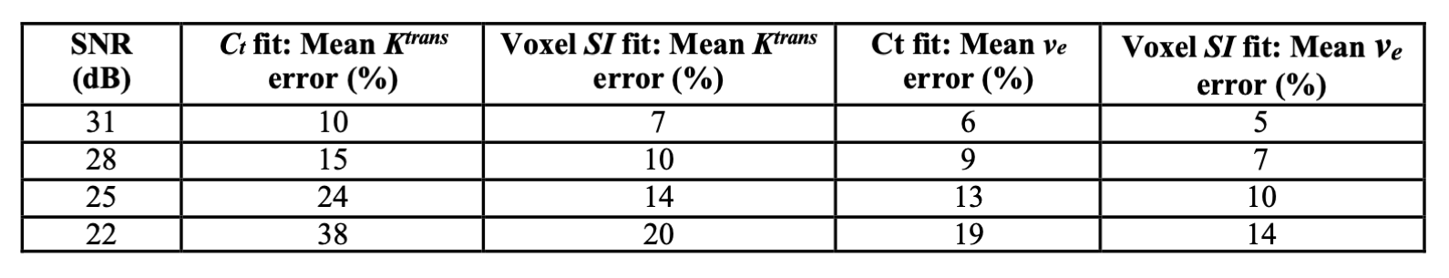
Table 1 shows the results of average parameter errors between fits to the simulated contrast agent concentration (Ct) curves and fits to the simulated signal intensity (SI) curves of simulated curves at the various signal to noise ratios (SNRs) tested. The noisiest simulated signal intensity curves (SNR 22 dB) showed the largest difference in errors between fits, as expected. The highest signal to noise curves (SNR 31 dB) showed the smallest difference in average parameter error between fits. Errors were larger for Ktrans than for ve as expected, as this parameter depends heavily on the peak and uptake portion of the contrast agent concentration curves. In all cases, mean errors were larger when the model was fit to concentration curves compared to signal intensity curve fits (p< 0.001.) Figure 2 shows an example of the Ktrans and ve parameter maps and noise maps (noise estimated as residuals to model fits) when the model is fit to signal intensity (top row) and concentration (bottom row) curves. For all patient data, parameter maps from model fits to signal intensity were smoother with significantly lower estimated noise levels, qualitatively indicating improved fits.Conclusion:
Simulations indicate that using signal intensity curves to perform fits of Kety-Tofts pharmacokinetic parameters should result in lower parameter errors due to image noise. Results also indicate that noisier images result in larger average error differences between fits to the contrast agent concentration and fits to the signal intensity. Based on our simulations and examination of a subset of patient breast cancer data, it is better to perform PK fits to signal intensity rather than relaxivity or contrast agent concentration time courses.Acknowledgements
We gratefully acknowledge the support of NCI U01CA142565, U01CA174706, and CPRIT RR160005.References
[1] Yankeelov TE, Gore JC. Dynamic Contrast Enhanced Magnetic Resonance Imaging in Oncology: Theory, Data Acquisition, Analysis, and Examples. Curr Med Imaging Rev. 2009 May 1;3(2):91-107.
[2] Tofts, P., & Parker, G. (2013). DCE-MRI: Acquisition and analysis techniques. In P. Barker, X. Golay, & G. Zaharchuk (Eds.), Clinical Perfusion MRI: Techniques and Applications (pp. 58-74). Cambridge: Cambridge University Press.
[3] Jarrett AM, Hormuth DA, Barnes SL, Feng X, Huang W, Yankeelov TE. Incorporating drug delivery into an imaging-driven, mechanics-coupled reaction diffusion model for predicting the response of breast cancer to neoadjuvant chemotherapy: theory and preliminary clinical results. Phys Med Biol. 2018 May 17;63(10):105015.
[4] Sorace, AG, Partridge, SC, Li, X, Virostko, J, Barnes, SL, Hippe, DS, Huang, W and Yankeelov, TE. Distinguishing benign and malignant breast tumors: preliminary comparison of kinetic modeling approaches using multi-institutional dynamic contrast-enhanced MRI data from the International Breast MR Consortium 6883 trial. J Med Imaging, 2018; 5(1): 011019.
Figures