Introduction

Susceptibility-Weighted Imaging (SWI) has become the gold standard technique for visualizing iron containing structures such as veins and cerebral microbleeds (CMBs) in the brain ¹. It takes advantage of the increase susceptibility weighting provided high-pass filtered phase images to further accentuate contrast in magnitude T2* weighted images through multiplication of a phase mask that highlights negative phase values of high frequency structures. The disadvantage of SWI is that it requires that either the raw kspace data or reconstructed phase images are saved along with the conventional magnitude images when the processing is not directly available on the scanner, hindering its widespread usage in the clinic. The method can also be prone to residual phase wrapping artifacts around air-tissue interfaces, limiting its application in diseases involving the temporal lobes. To address these limitations, the goal of this study was to train a deep convolutional neural network to learn the SWI contrast from T2*-weighted magnitude images and assess the performance of the resulting network on CMB detection.

Methods

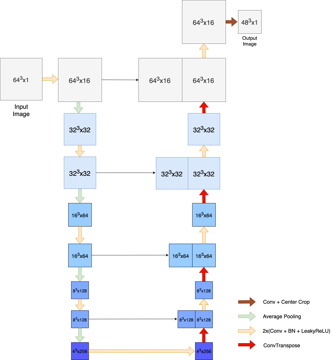
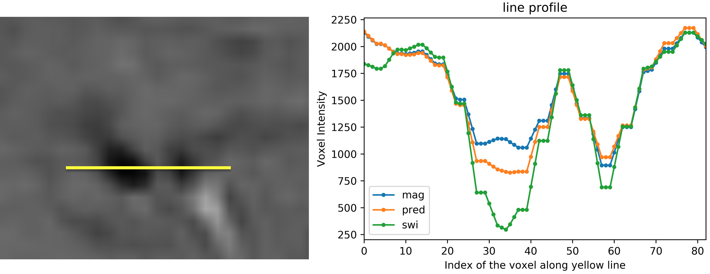
Subjects and data acquisition: 3D T2*-weighted gradient echo (GRE) magnitude and phase MRI data from 146 patients with treated gliomas who developed radiation-induced CMBs were collected using a 3T GE scanner with 8-channel head coil (TE/TR=28/46ms, flip angle=20⁰, FOV=24cm, 0.625x0.625x2mm resolution, R=2 acceleration). SWI images were generated using traditional processing methods.
Network implementation and evaluation: Networks were implemented in Pytorch 1.5.1 and trained using NVIDIA GeForce RTX 2070, 8GB. We used a Least Squares Generative Adversarial Network (LSGAN) as a deep learning technique to produce synthetic SWI data. The advantage of this approach is that it can capture high frequency edges and structures which are important in this task ². Figure 1 shows the U-Net generator network. 3D patches of T2*-weighted magnitude images, excluding regions of residual phase artifacts on SWI, were used as inputs in the training. Voxel intensity values of all images were normalized to [0, ~1] by dividing their intensities by 5 times of the mode values of each image. We used 122 scans for training the network, 4 scans for validation, and 20 scans in testing. Hyperparameter values were initialized from Chen et al ³; learning rate, batch size and number of channels were further optimized using Bayesian Optimization on the validation set. An Adam optimizer was used with initial learning rate of 0.0085, beta1= 0.5, beta2 = 0.999. A combination of mean absolute error loss and adversarial loss was used for the generator. Models were trained for 400000 iterations. Structural Similarity Index (SSIM) was used to evaluate the performance of the model on the test data. Histograms of image intensity, SSIM values, and line profiles of individual CMBs were compared between magnitude, original SWI, and predicted synthetic SWI images.

Results and Discussion

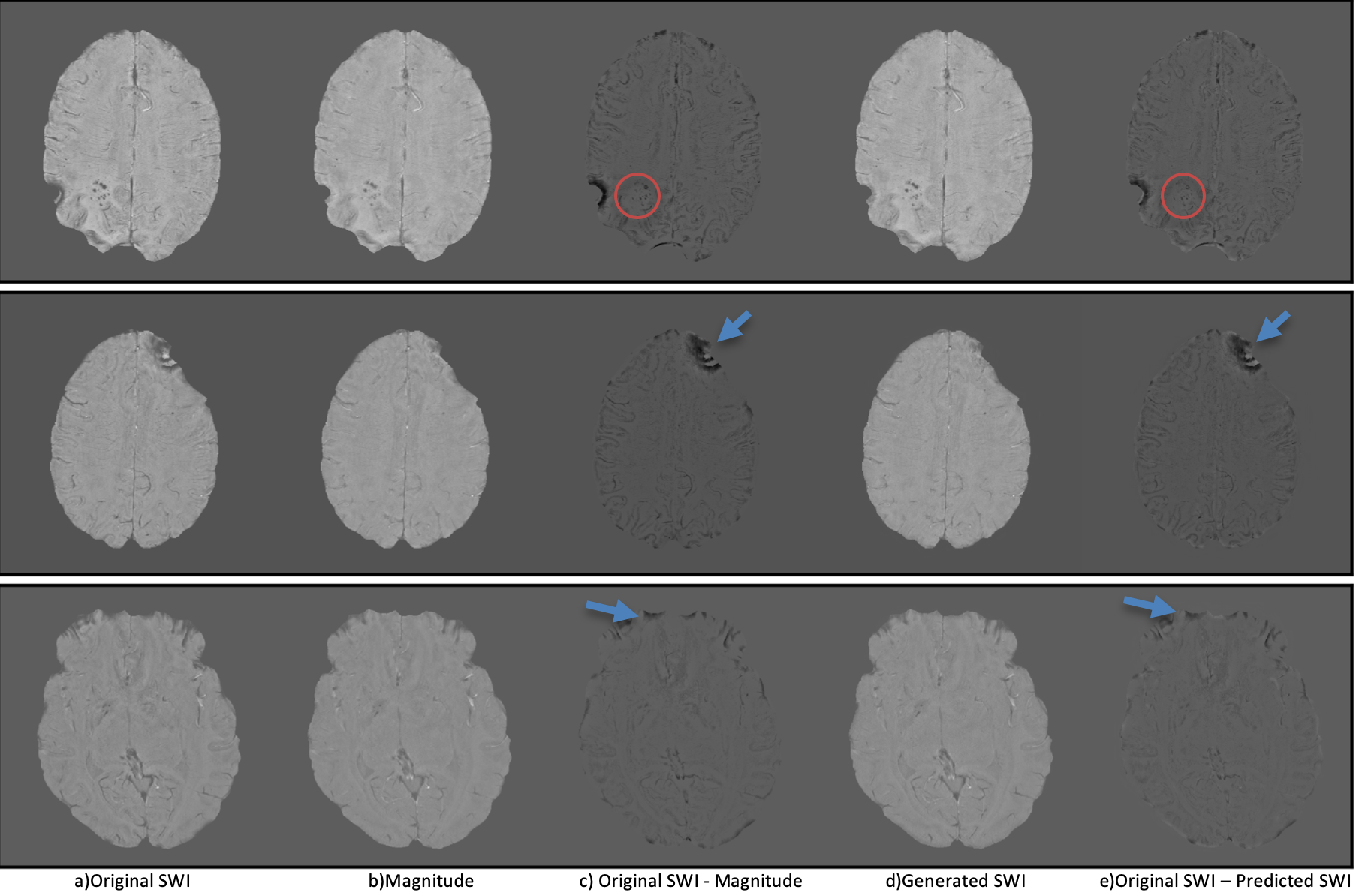
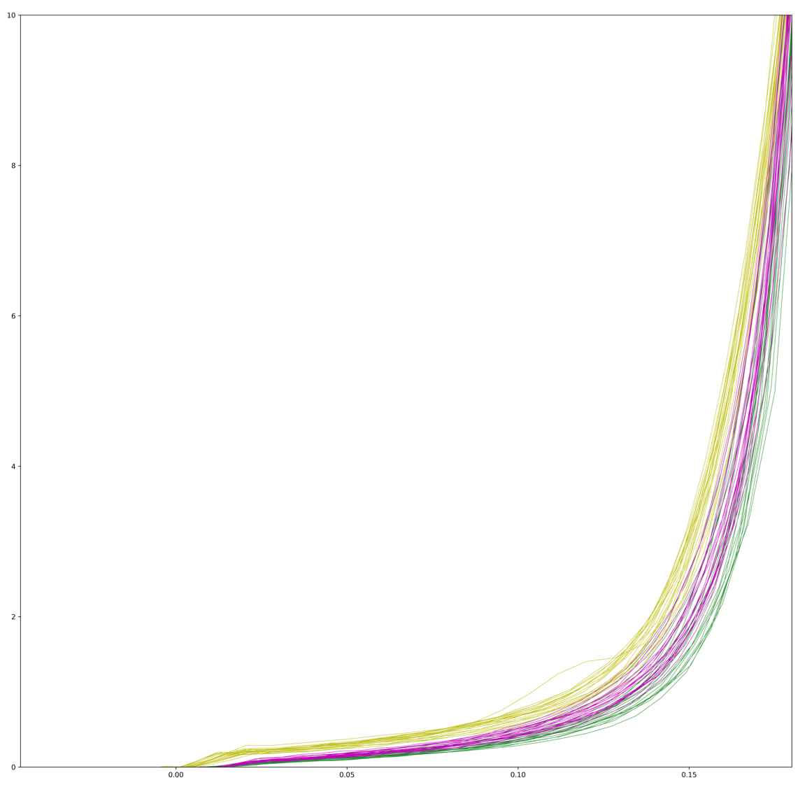
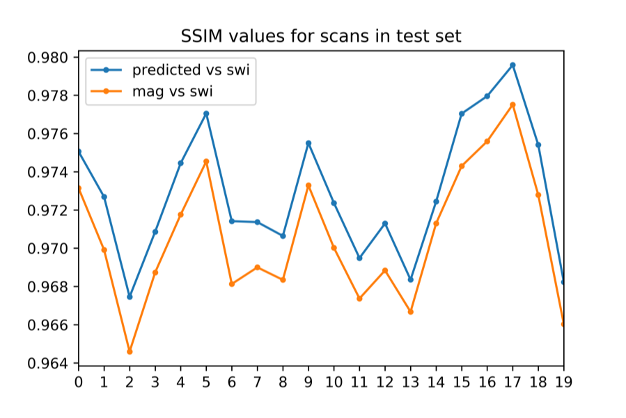
Figure 2 compares representative images of magnitude, original SWI, predicted SWI and corresponding difference images. CMBs are more visible in the difference image of original SWI and magnitude image than they are in difference image of original and predicted SWI. This suggests that CMB contrast in predicted image is more similar to the original SWI. Residual phase artifacts present in the original SWI image have also been removed in the predicted SWI (Figure 2, second and third rows). This is because slices with artifacts on the original SWI images were excluded in the training. Figure 3 shows the left tail of the distribution of voxels affected by the SWI processing. A slight shift to the left (more negative intensities) is observed with our predicted SWI images compared to the magnitude images, but not as large of a shift as seen with the original SWI. SSIM values between the original and predicted SWI were higher than the SSIM values between original SWI and magnitude images for all test images as shown in Figure 4. From the line profile analysis, we observed that voxel intensity values of the predicted synthetic SWI images were closer to the original SWI than the magnitude images for a large CMB. Taken together, these findings suggest that our deep learning model is able to improve CMB contrast from just magnitude images

Conclusion

Our findings suggest that it is possible for a deep learner to learn the added susceptibility contrast produced with SWI. Although we were able to generate synthetic SWI images that were more similar in contrast to the original SWI image than magnitude image, there is room to further increase the contrast to more closely match standard SWI processing. Still, our method provides the additional advantage of residual phase artifact removal and can be beneficial in circumstances when phase data has not been saved.

Acknowledgements

This research was supported by NIH NICHD grant R01HD079568.