Introduction

Dynamic contrast-enhanced magnetic resonance (DCE-MR) imaging is an important clinical and research tool for cancer imaging.¹ DCE-MR imaging uses an injected contrast agent to investigate the microcirculation and the disruption of the blood-brain barrier by estimating perfusion and permeability maps. However, a necessary step for modeling the quantitative maps requires the extraction of a vascular function (VF).² Commonly this step is performed manually in many DCE-MR analysis, making it both time-consuming and prone to human error. In the brain, both arteries and veins have been used to determine a VF.^3,4,5 Here, we present a deep learning approach to automatically estimate a region over the transverse sinus on 4D DCE-MR images in order to estimate a VF. A unique property of this problem is that many regions in the vein yield similar vascular functions. Thus, the problem of estimating a VF can be simplified by finding a region over the vein that need not match the location of the manually selected region used to train the model.

Materials and Methods

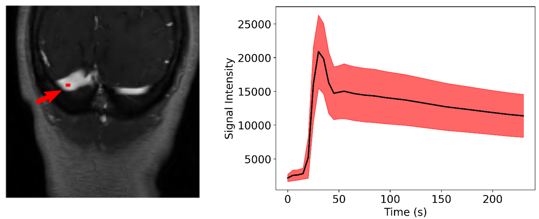
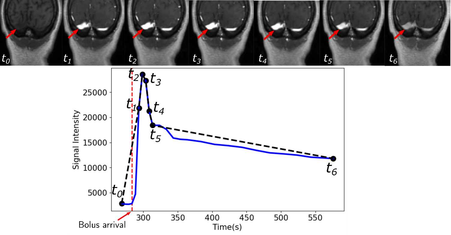
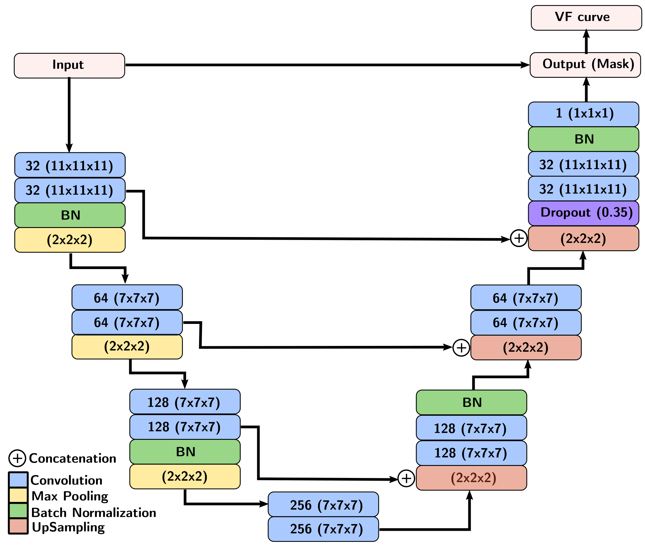
A total of 43 patients with glioblastoma were enrolled in this study (age: 59 ± 9.8 years [mean±standard deviation], 19 male). They were scanned post-resection using a protocol approved by our local research ethics board. A total of 155 baseline and follow-up DCE-MR image volumes were obtained from these patients. DCE-MR acquisition parameters were TR = 5 ms, TE = 1.9 ms, field-of-view of 240 mm × 240 mm, pixel size of 0.94 mm × 1.0 mm, and slice thickness of 2.0 mm. The DCE-MR image volumes were randomly divided into 100 (64.5%) volumes for training, 23 (14.8%) volumes for validation, and 32 (20.6%) volumes for testing. All images were normalized, on a per volume basis, by their maximum intensity to lie within the range [0,1]. The VF was extracted manually on the dynamic images by drawing a region of interest (ROI) on a coronal view containing the transverse sinus (Fig. 1). Because the VF had a priori defined characteristics (i.e., a sharp signal increase, followed by a short-duration maximum, and a slow decrease (Fig. 1)), the temporal dynamics of the data volume were undersampled for memory optimization. The VF sampling algorithm was based on the bolus arrival (BAT): One sample before the bolus arrival, five during bolus passage, and a seventh during the contrast wash-out (Fig. 2). The seven image volumes were then cropped to remove portions of the background that did not contribute to the VF and the temporal information was encoded into the seven channels of the input image.
We used a 3D U-net architecture⁶ with three levels. The encoder consisted of repeated 11×11×11 and 7×7×7 padded convolutions, each followed by a leaky rectified linear unit (leaky ReLU,⁸ scale parameter=0.3), batch normalization, and a 2×2×2 max pooling operation. After each downsampling, the number of filters was doubled. The decoder consisted of upsampling and concatenation operation with successive 7×7×7 and 11×11×11 padded convolutions, each followed by a leaky ReLU, and a final layer 1×1×1 padded convolution followed by a sigmoid activation function (Fig. 3). As different regions over the transverse sinus can yield similar vascular functions, the predicted region does not need to match the location of the manually selected region. However, the separation between predicted and manual regions should be small. Thus, our loss function consists of two terms: a spatial term (distance between the predicted and manual region centers of mass, CoM, see coordinate definition in Fig. 4) and a temporal term (mean square error (MSE) between the sampled time signals). We evaluated the VF curve quality and how close our predicted region was to the manual region.

Results

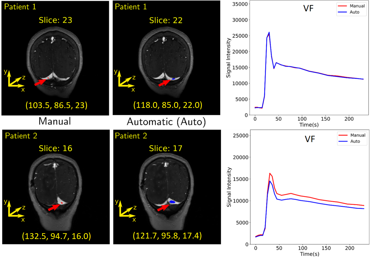
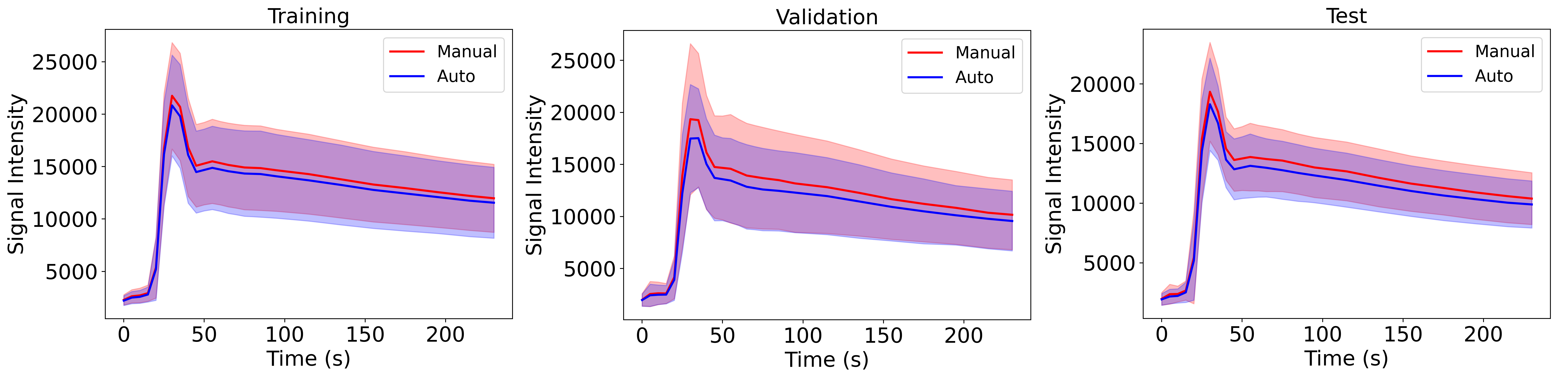
For training, validation, and testing we achieved MSE of 0.0028, 0.0035 and 0.0020, and CoM difference of 10.4, 5.4, and 11.4 voxel, respectively. The average absolute error in the CoM coordinates were (training: 9.12±8.16, 2.91±3.98, 1.57±1.65 voxels), (validation: 4.08±3.13, 1.68±1.66, 1.43±1.68 voxels), and (testing: 10.47±8.10, 2.4±2.61, 1.26±1.37 voxels). The overall prediction performance was good (Fig. 5). Examples of VF estimation for different patients are shown in Fig. 4.

Discussion

The larger variance on the CoM x and y coordinates is due the fact that different regions over the transverse sinus can yield similar vascular functions, as shown in Fig. 5. Lower variance of the CoM z coordinate suggests that the predicted region was close to the slice of the manual region. The low MSE confirms that the predicted VF followed the same characteristics as the manual VF. Our VF prediction was close to the manual VF (Fig. 4).

Conclusion

We demonstrated an automatic deep learning method can estimate a region over the transverse sinus in DCE-MR images can be used to identify a VF. Our method differs from other proposed deep learning methods,⁷ in that our model concurrently works with the spatial and temporal information, reducing the complexity of the network architecture. Our results demonstrated that our model generalizes well for unseen data and can be used to generate suitable VF. Next, we plan to compute and compare permeability maps using the manual and automatic vascular functions proposed in this work.

Acknowledgements

University of Calgary - Eyes High Scholar Award.