3251

Reduction of J-difference Edited Magnetic Resonance Spectroscopy Acquisition Times Using Deep Learning

Roberto Souza^1,2, Jordan McEwen³, Carissa Chung³, and Ashley D. Harris^2,4
¹Electrical and Computer Engineering, University of Calgary, Calgary, AB, Canada, ²Hotchkiss Brain Institute, Calgary, AB, Canada, ³Biomedical Engineering, University of Calgary, Calgary, AB, Canada, ⁴Radiology, University of Calgary, Calgary, AB, Canada

Synopsis

Magnetic Resonance Spectroscopy (MRS) non-invasively acquires in-vivo data on the chemical composition of localized tissue samples. MRS acquisitions are lengthy because they often require the acquisition of several averages to obtain a spectrum with a sufficient signal to noise ratio (SNR). This issue is augmented in J-difference edited MRS in which the analyzed spectrum is generated as the difference between sub-spectra in which editing pulses have been applied to selectively refocus the coupling of the target metabolite. In this work, we investigate the reduction of J-difference edited MRS acquisition times using deep learning.

INTRODUCTION

Magnetic Resonance Spectroscopy (MRS) is used to non-invasively quantify metabolites in vivo. In order to acquire high quality data, many transients or averages are acquired and then averaged for metabolite quantification, making MRS acquisitions long and prone to motion artifacts. Furthermore, metabolites with low concentrations that are overlapped by more abundant metabolites cannot be readily identified within a conventional MRS spectrum¹. For example, the 3 ppm GABA peak is overlapped by the more concentrated metabolite creatine².

The most widely used approach to overcome these challenges is J-difference editing (e.g., MEGA- or BASING)¹. In a J-difference edited experiment, a frequency selective editing pulse is applied refocus the coupling of a particular metabolite. This editing pulse does not affect the other overlapping metabolites at the same frequency. For example, a frequency selective editing pulse at 1.9 ppm will refocus the coupling of the 3 ppm GABA without affecting the overlapping creatine signal. The difference between the edited (ON) and the non-edited pulses (OFF) results in the J-difference edited spectrum. J-difference editing is highly noise sensitive because it depends on the subtraction of two low SNR measurements and requires measuring more transients during acquisition, making acquisition slower.

In this work, we demonstrate the potential for Deep Learning to denoising edited-MRS to enable in shorter acquisition times. For clarity, transient will refer to a data acquired from a single repetition (TR) while average will refer to averaged groups of transients.

METHODS

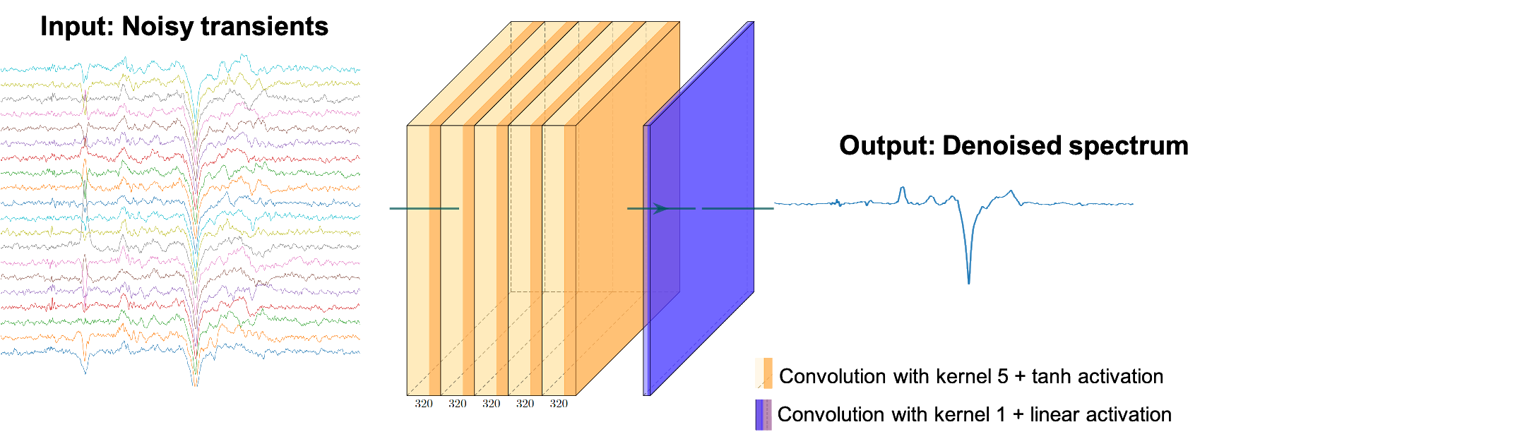
We used 27 GABA-edited MRS acquisitions from the BigGABA repository³ (3T, GE scanners, TR/TE = 2s/68 ms, 320 transients, 14 ms editing pulse at 1.9 ppm in the edit-ON condition). Data were preprocessed including spectra registration for frequency and phase correction with Gannet3⁴.

We used a flat Convolutional Neural Network (CNN) with five layers with 320 filters with a kernel size of 5 and a hyperbolic tangent activation. The final layer has one convolution with a kernel size of 1 and a linear activation. The model architecture is depicted in Figure 1. The inputs are the measured transients, and the output is the denoised spectrum. The loss function used to train the model was the mean squared error.
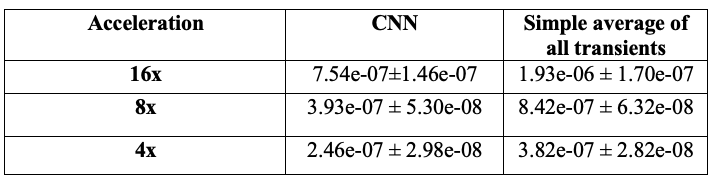
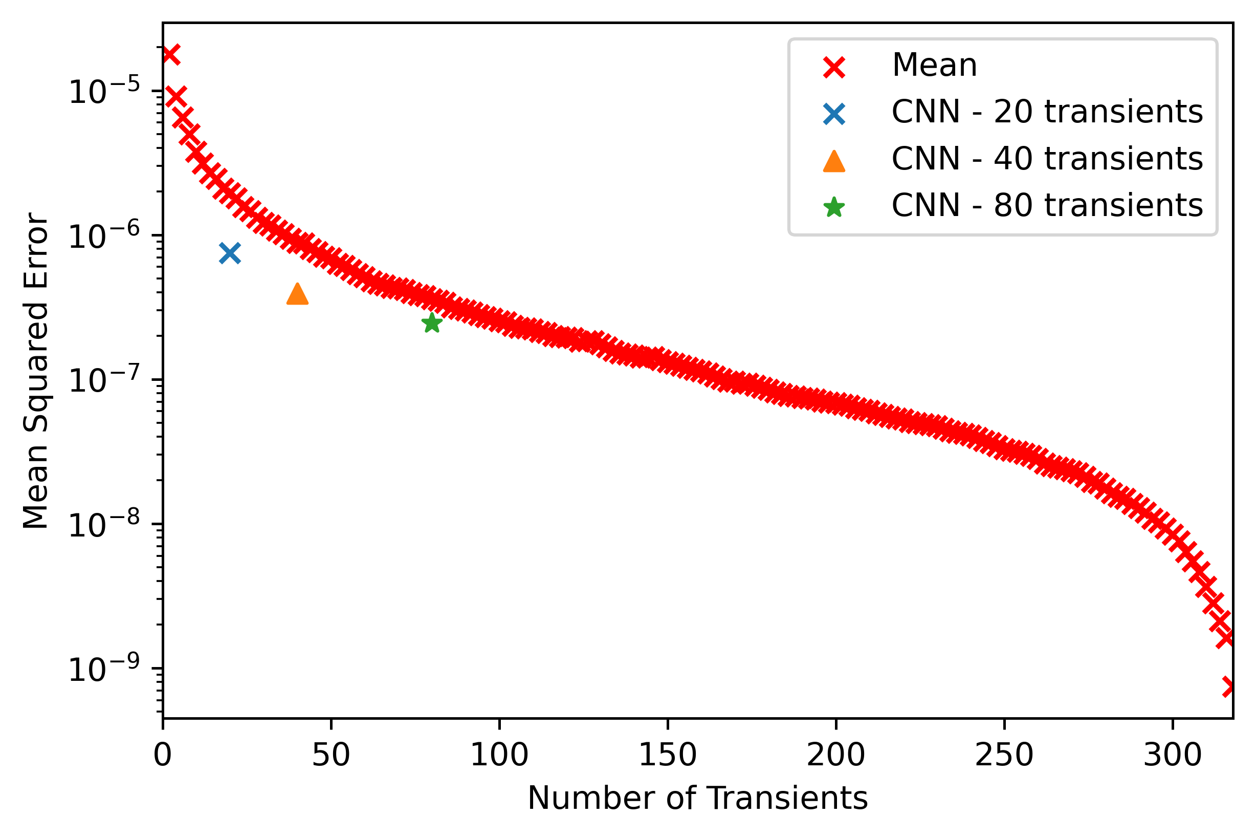
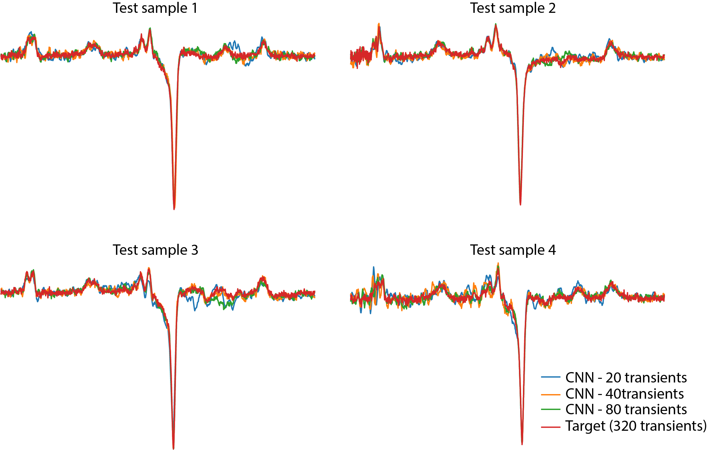
Eighteen datasets were used for training, five for validation, and four for testing the model. For data augmentation purposes, the ON and OFF transients were treated as different samples (i.e., processed independently), and the transients were randomly selected during training epochs. The subtraction of the OFF transients' prediction from the ON transients' prediction results in the denoised difference spectrum. The reference for the model is the spectrum computed from the 320 transients. The CNN results were compared against averaging subsets of the full set of 320 transients. We report the mean squared error (MSE) computed from 10 random permutations of the transients across the samples in the test set. We evaluated three different acceleration rates: 4x (80 transients, CNN-80), 8x (40 transients, CNN-40), and 16x (20 transients, CNN-20).

RESULTS

The MSE results for the different CNN models are summarized in Figure 2. The CNN model results outperformed simple averaging of the transients in all experiments. The MSE curve (Figure 3) was obtained by increasing the number of averages included the final spectrum and errors of the different CNN models relative to averaging all 320 transients are shown. The CNN-20 model achieved an error comparable to averaging 46 transients (23 edit-ON and 23 edit-OFF transients). The CNN-40 model achieved an error equivalent to averaging 74 transients, and the CNN-80 model achieved an error similar to averaging 102 transients.

DISCUSSION

Our investigation using a flat CNN model with a relatively low number of trainable parameters (~2M) indicated that it could serve as a denoiser for MRS data and potentially reduce acquisition times by collecting fewer transients.

While designing our methods, we experimented using a residual CNN, which is known to mitigate the vanishing gradient problem during training. For MR image reconstruction (which is analogous to the current MRS denoising problem) residual CNNs achieve superior results compared to CNNs without the residual connection⁵. Interestingly, the model without the residual connection achieved best results, which we hypothesize is due to the noisy nature of the transients.

An important factor to consider is that we kept the number of filters in the CNN architecture constant, but the dimensionality of the inputs vary according to the acceleration rate being trained. Increasing the network capacity could potentially improve the results. However, due to the limited data available and the risk of overfitting, we did not investigate increasing the network capacity but with the addition of data we will investigate network capacity in future.

CONCLUSION

Our results on a relatively small dataset showed that deep learning models hold the potential to greatly reduce J-difference-edited MRS acquisition times. These results suggest that CNNs can decrease acquisition time for GABA-edited MRS by at least half as the 8x and 16x acceleration results compared to simple averaging of twice as many transients.

Acknowledgements

This work is supported by the Natural Sciences and Engineering Research Council of Canada (NSERC, RGPIN-2017-03875) and the Canada Research Chairs Program.

References

1. Harris, Saleh and Edden, "Edited 1 H Magnetic Resonance Spectroscopy In Vivo: Methods and Metabolites," Magnetic Resonance in Medicine, vol. 77, pp. 1377-1389, 2017.

2. Near, Evans, Puts, Barker and Edden, "J-difference editing of GABA: simulated and experimental multiplet patterns," Magnetic Resonance Medicine, vol. 70, no. 5, pp 1183-1191, 2013.

3. Mikkelson et al., "Big GABA: Edited MR spectroscopy at 24 research sites.," Neuroimage, vol. 52, pp. 32-45, 2017.

4. Edden, Puts, Harris, Barker and Evans, "Gannet: A batch-processing tool for the quantitative analysis of gamma-aminobutyric acid-edited MR spectroscopy spectra," Journal of Magnetic Resonance Imaging, vol. 40, pp. 1445-1452, 2014.

5. Lee, Yoo, and Ye, "Deep residual learning for compressed sensing MRI," In 2017 IEEE 14th International Symposium on Biomedical Imaging, pp. 15-18. IEEE, 2017.

Figures

Figure 1. Architecture of the CNN model used in the experiments. The model processes the ON and OFF transients separately and subtracts the results to obtain the final J-difference edited spectrum.

Figure 2. Mean squared error results of the CNN model compared against averaging the transients. Mean ± standard deviation results are reported. The results were obtained from averaging 10 random permutations of transients across the test set. The reference used to compute the metrics was the average of all 320 acquired transients. In all cases, the mean square error of the CNN is substantially lower than a simple average of the included transients.

Figure 3. Mean squared error results obtained by averaging random permutations of different number of transients and for the different CNN models trained. The CNN-20 model achieved an error compared to averaging 46 transients. The CNN-40 model achieved an error compared to averaging 74 transients. The CNN-80 model achieved an error compared to averaging 102 transients.

Figure 4. Sample spectra reconstructed by the different CNN models for the different samples in the test set.

Proc. Intl. Soc. Mag. Reson. Med. 29 (2021)

3251