3134

Deep Linear Modeling of Hierarchical Functional Connectivity in the Human Brain

Wei Zhang¹, Eva M Palacios¹, and Pratik Mukherjee¹
¹UCSF, San Francisco, CA, United States

Synopsis

To better map hierarchical brain connectivity networks, we introduce a novel class of deep (multilayer) linear models of fMRI that bridge the gap between conventional methods such as independent component analysis and more complex deep nonlinear models. These deep linear models do not require the manual hyperparameter tuning, extensive fMRI training data or high-performance computing infrastructure needed by deep learning, such as convolutional neural networks, and their results are more explainable from their mathematical structure. These benefits gain in importance as continual improvements in the spatial and temporal resolution of fMRI reveal more of the hierarchy of spatiotemporal brain architecture.

Purpose

The human brain exhibits hierarchical modular organization, which is not depicted by conventional fMRI functional connectivity reconstruction methods such as independent component analysis (ICA)¹. Current nonlinear models such as the Deep Belief Network (DBN)² have several disadvantages, requiring: 1) large training samples; 2) high-performance computational resources, e.g., GPUs; 3) manual tuning of hyperparameters; 4) time-consuming training process; 5) non-convergence to the global optimum; and 6) “black box” results that lack explainability. To better map hierarchical brain connectivity networks (BCNs), we propose a novel class of deep (multilayer) linear models that overcome the shortcomings of nonlinear approaches, since they are fast even on conventional CPUs with hyperparameters that can be automatically determined and with convex optimization functions that are guaranteed to converge.

Methods

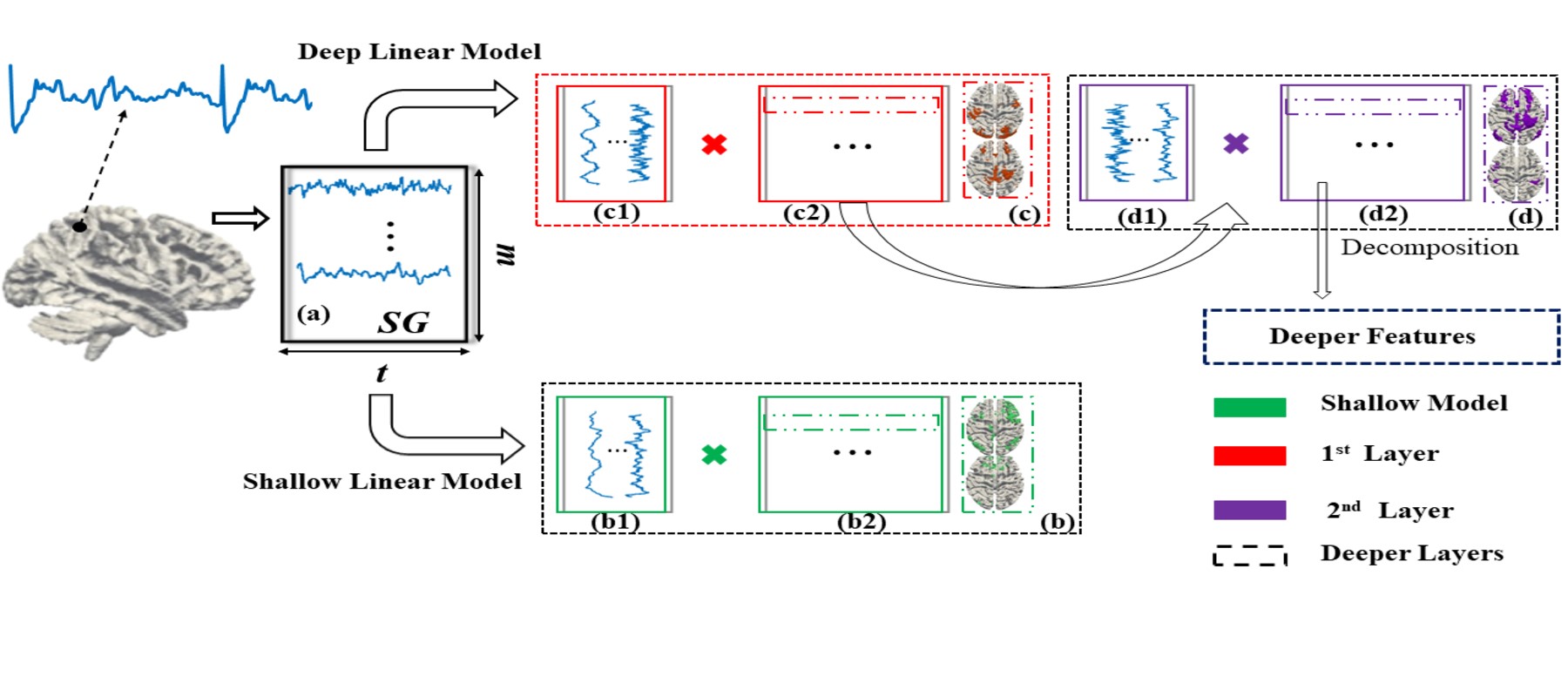
Three deep linear models are multilayer variants of Sparse Dictionary Learning (SDL)³, Non-Negative Matrix Factorization (NMF)⁴ and Fast ICA (FICA)⁵. A fourth deep linear model, Deep Matrix Fitting (MF), incorporates rank reduction for data-driven hyperparameter determination and the distributed optimization function Alternating Direction Method of Multipliers (ADMM)⁶ that is well suited for compositional approaches to hierarchical systems analysis (Figure 1). More complete descriptions of each method can be found in the full bioRxiv report: https://biorxiv.org/cgi/content/short/2020.12.13.422538v2

1. Deep Matrix Fitting: Deep MF is a deep SDL (described below) with the additional mechanism to automatically determine all crucial hyperparameters via rank reduction. The hierarchical dictionary of each layer is equivalent to the weight matrix in ICA and DBN. The hierarchical spatial features of each layer are denoted as a correlation matrix, as are the noise matrices. We assume the spatial features of each layer can be decomposed as the dictionary and spatial features of the next layer, in order to implement the compositional deep linear framework (Figure 1). A rank reduction operator automatically estimates the hyperparameters of Deep MF in data-driven fashion, including the maximum number of layers. For the sparse trade off, two parameters control the sparsity levels of background components (noise) and spatial features.

2. Deep Sparse Dictionary Learning: For the first layer of Deep SDL, the input matrix is decomposed into the product of an incomplete or over-complete dictionary basis matrix (each atom representing a time series) and a feature matrix (representing this network’s spatial volumetric distribution). For each successive layer (Figure 1), the current features matrix is treated as an input matrix to be continuously decomposed, optimized using gradient descent (GD). An interesting property of Deep SDL is the ability to perform over-complete decomposition (number of features > number of time points).

3. Deep Fast Independent Component Analysis: In each layer of Deep FICA, the previous independent component (IC) matrix is the input signal matrix that will be decomposed using principal component analysis (PCA) and the Fixed-Point algorithm continuously (Figure 1). Deep FICA concentrates on extracting spatially independent features and can only solve the incomplete decomposition problem (number of features < number of time points) but not over-complete decomposition.

4. Deep Non-negative Matrix Factorization: Deep NMF focuses on the decomposition of the non-negative multivariate data matrix into hierarchical factors similarly to Deep FICA but with a non-negative data constraint and with a different but equally fast update policy.

Results

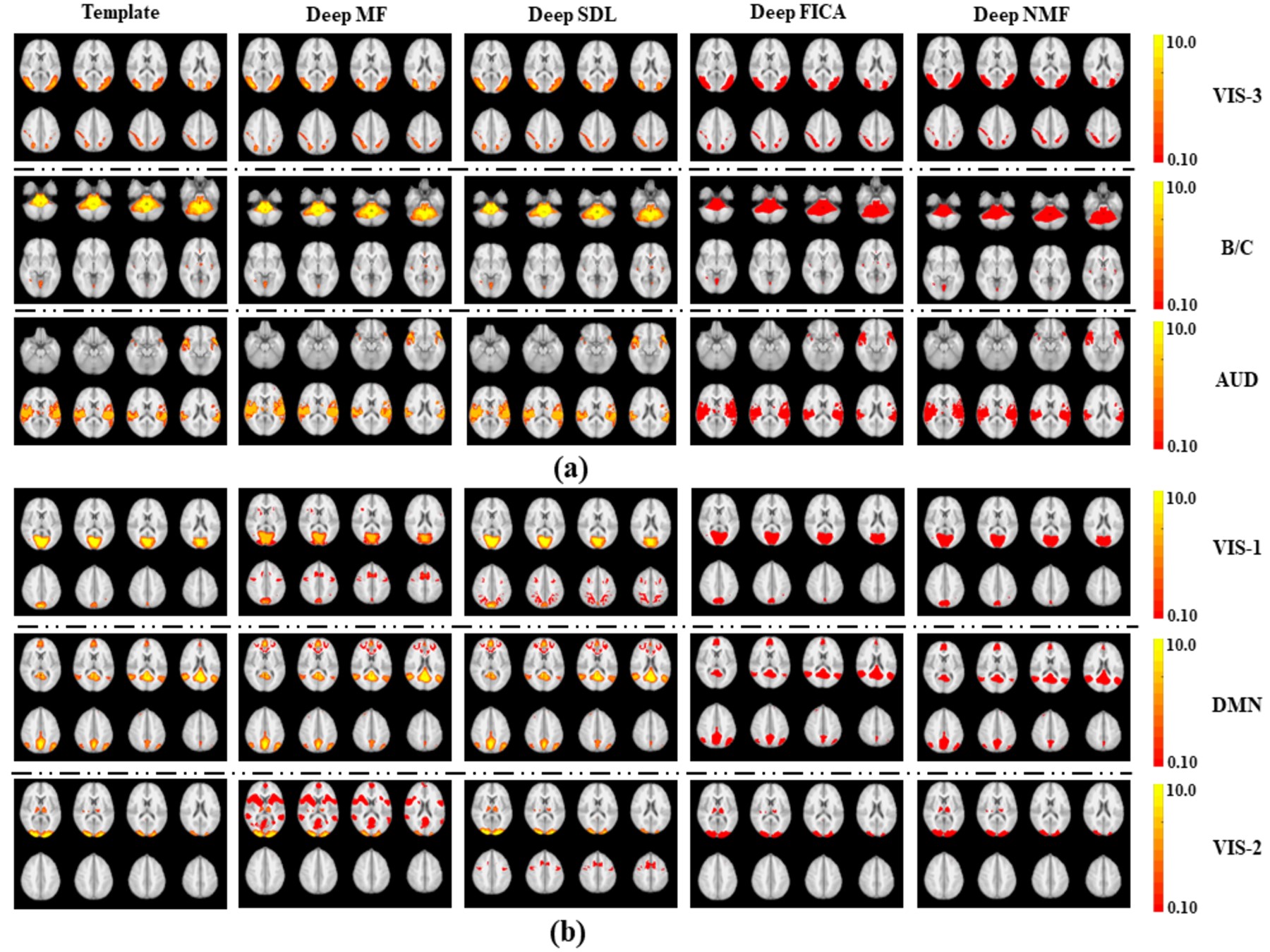
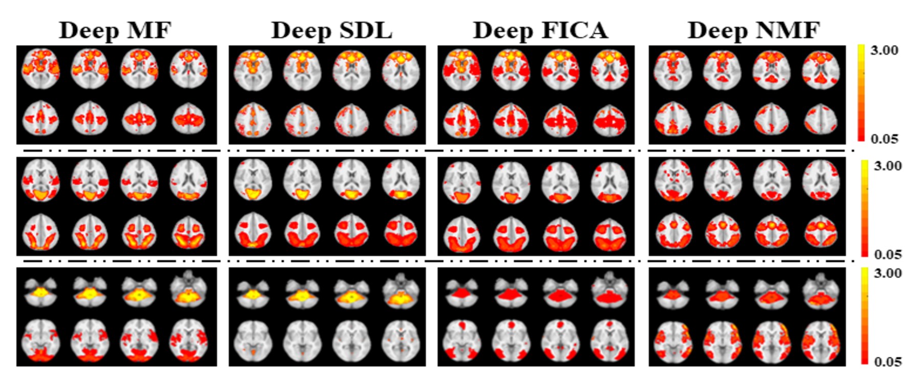
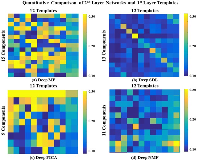
Using a previously described fMRI simulation with ground truth template BCNs⁷, we find that all four deep linear models can accurately reconstruct all twelve BCNs in their 1st layer, with examples from six of the 12 1st layer BCNs shown in Figure 2. Deep NMF and Deep FICA had the best spatial similarity to the templates, whereas Deep MF and Deep SDL had the best intensity similarity to the templates.

Several 2nd layer BCNs were conserved across all four deep linear models and demonstrated neurobiological face validity, for example, combined nodes of the executive control network, salience network and default mode network (Figure 3, top row). The salience network is known to modulate the anticorrelated activity of the executive control and default mode networks. Considerable spatial variation across deep linear models was observed for other 2nd layer features (Figure 4).

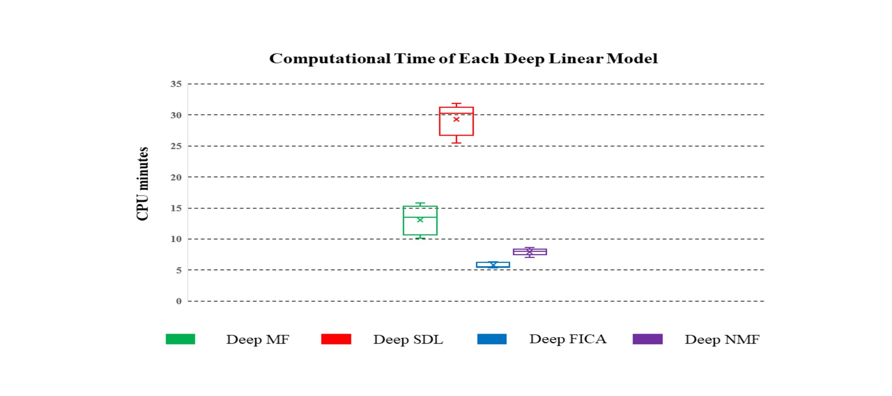
Of the four models, Deep MF produced the best combination of spatial matching, intensity matching and computational efficiency, the latter shown in Figure 5.

Discussion

Since these deep linear models do not require large training datasets nor specialized computing infrastructure, they can be easily applied to clinical research with the potential to generate novel functional connectivity biomarkers of neurodevelopmental, neurodegenerative, and psychiatric disorders⁸, including for diagnosis, prognosis and treatment monitoring. This is particularly significant given the recent observation that neuropathology and psychopathology often affect low-level network connectivity differently than high-level network connectivity. For example, many different psychiatric disorders have been found to decrease lower-order sensory and somatomotor network connectivity in a uniform manner across patients^9,10, while increasing distinctiveness among patients in networks at higher levels of the hierarchy^8,11. Higher fMRI sensitivity and spatial resolution will enable mesoscale functional imaging that supports more 1st layer components of deep linear models to uncover subnetworks of the BCN templates used in this work. This will also permit the use of deeper models for principled unsupervised dynamic functional connectivity mapping that reveals ever more of the human brain’s hierarchical modular organization.

Acknowledgements

This work was supported by the U.S. National Institutes of Health [R01
MH116950, U01 EB025162] and U.S. Department of Defense [W81XWH-14-2-0176].

References

1. Calhoun, V.D., Adali, T., Pearlson, G.D., Pekar, J.J. (2001). A method for making group inferences from functional MRI data using independent component analysis. Human Brain Mapping, 14:140–151.

2. Zhang, W., Zhao, S., Hu, X., Dong, Q., Huang, H., Zhang, S., ... & Liu, T. (2020). Hierarchical Organization of Functional Brain Networks Revealed by Hybrid Spatiotemporal Deep Learning. Brain Connectivity, 10:72-82.

3. Lv, J., Jiang, X., Li, X., Zhu, D., Zhang, S., Zhao, S., Chen, H., Zhang, T., Hu, X., Han, J. (2015). Holistic atlases of functional networks and interactions reveal reciprocal organizational architecture of cortical function. IEEE Transactions on Biomedical Engineering, 62:1120-1131.

4. Trigeorgis, G., Bousmalis, K., Zafeiriou, S., & Schuller, B. W. (2016). A deep matrix factorization method for learning attribute representations. IEEE Transactions on Pattern Analysis and Machine Intelligence, 39:417-429.

5. Hyvarinen, A. (1999). Fast and robust fixed-point algorithms for independent component analysis. IEEE transactions on Neural Networks, 10(3), 626-634.

6. Shen, Y., Wen, Z., & Zhang, Y. (2014). Augmented Lagrangian alternating direction method for matrix separation based on low-rank factorization. Optimization Methods and Software, 29:239-263.

7. Zhang, W., Lv, J., Li, X., Zhu, D., Jiang, X., Zhang, S., ... & Liu, T. (2019). Experimental Comparisons of Sparse Dictionary Learning and Independent Component Analysis for Brain Network Inference from fMRI Data, IEEE Transactions on Biomedical Engineering, 66:289-299.

8. Parkes, L., Satterthwaite, T. D,, Bassett, D. S. (2020). Towards precise resting-state fMRI biomarkers in psychiatry: synthesizing developments in transdiagnostic research, dimensional models of psychopathology, and normative neurodevelopment. Curr Opin Neurobiol, 65:120-128.

9. Elliott, M. L., Romer, A., Knodt, A. R., Hariri, A. R. (2018). A connectome-wide functional signature of transdiagnostic risk for mental illness. Biol Psychiatry, 84:452-459.

10. Kebets, V., Holmes A. J., Orban, C., Tang, S., Li, J., Sun, N., Kong, R., Poldrack, R. A., Yeo, B. T. T. (2019). Somatosensory-motor dysconnectivity spans multiple transdiagnostic dimensions of psychopathology. Biol Psychiatry, 86:779-791.

11. Kaufmann, T., Alnæs, D., Doan, N. T,, Brandt, C. L., Andreassen, O. A,, Westlye, L.T. (2017). Delayed stabilization and individualization in connectome development are related to psychiatric disorders. Nat Neurosci, 20:513-515.

Figures

Figure 1. Deep linear model (shown as (c), (d)) versus shallow linear model (shown as (b)). (a) SG represents the input fMRI signal matrix, containing the t time points and m voxels. (c1) and (d1) represents the weight matrix/dictionary identified via SG of 1st and 2nd layer, respectively. (c2) and (d2) represents the feature matrix of 1st and 2nd layer, respectively. The dashed blue rectangle indicates the deeper features beyond the 2nd layer.

Figure 2. Comparison of six representative 1st layer networks from all four deep linear models (presented in the second to fifth column) with the ground truth templates (presented in the first column) from simulated fMRI data. (a) Three networks illustrate better intensity matching to the templates by Deep MF and Deep SDL than by Deep FICA or Deep NMF. (b) Three networks show better spatial matching to the templates by Deep FICA and Deep NMF than Deep MF or Deep SDL. Auditory Network: AUD. Brainstem/Cerebellum: B/C. Default Mode Network: DMN. Visual networks: VIS-1, VIS-2, VIS-3.

Figure 3. Comparisons of BCNs derived from the 2nd layer of Deep MF, Deep SDL, Deep FICA and Deep NMF. Each column includes three representative 2nd layer networks from a deep linear model, matched across models in each row. The top row shows a high-level network similar to the executive control network, but also including nodes of the salience network and/or default mode network. The middle row demonstrates coupling of visual networks with the dorsal attention network into a higher-level network. The bottom row links visual networks with cerebellar function.

Figure 4. Spatial similarity matrices of BCNs from the 2nd layer of Deep MF, Deep SDL, Deep FICA and Deep NMF to the 1st layer templates. Each element represents the spatial similarity of the identified components and the templates; (a), (b), (c) and (d) are Deep MF, Deep SDL, Deep FICA and Deep NMF, respectively. The rows represent the identified 2nd layer BCNs and the columns represent the 12 ground truth templates of the simulated experiment.

Figure 5. Comparisons of computation time of 10 independent runs, using the same number of iterations and the same simulated fMRI dataset for Deep FICA (blue), Deep SDL (red), Deep MF (green) and Deep NMF (purple). The box plots give the CPU time in minutes for the 10 runs.

Proc. Intl. Soc. Mag. Reson. Med. 29 (2021)

3134