3131
Mapping of phase-space dynamics for fMRI data1Department of Electrical and Computer Engineering, University of California,Riverside, Riverside, CA, United States, 2Department of Bioengineering, University of California,Riverside, Riverside, CA, United States
Synopsis
This work aims to map the dynamics of resting state fMRI data. With phase space embedding, we reconstructed the phase portrait of BOLD signal and calculated the sum of the length of the edges of the convex hull to capture the dynamics of fMRI BOLD time courses. Our statistical parametric maps on multiple datasets of mental disorder suggest that SE could be a viable disease biomarker.
Introduction
The human brain is a complex neurobiological system with nonlinear dynamics that have not been fully explored. With resting resting-state functional magnetic resonance imaging (rs-fMRI), the present study employed phase space embedding to reconstruct phase portraits for blood oxygen level dependent (BOLD) signals and mapped the phase space dynamics with the sum of the length of the portrait edges (SE). We applied this method on datasets of two mental disorders, i.e., schizophrenia (SZ) and autism spectrum disorder (ASD). The resultant statistical parametric maps based on SE demonstrated that the present method is promising in characterizing the instability of BOLD signals in patients.Methods
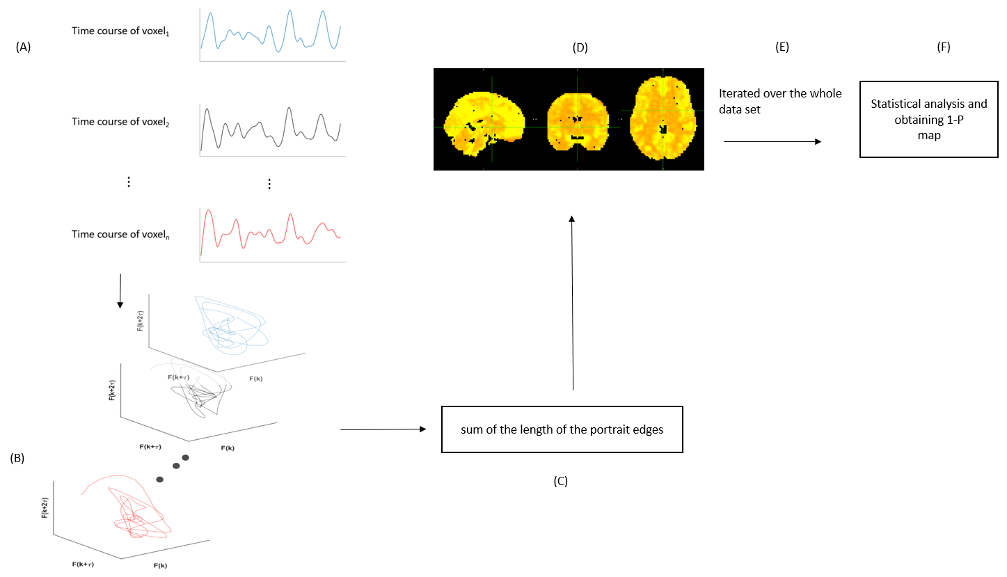
Phase space embedding and feature extraction of phase portraitWe constructed the phase space for the BOLD signal of a single voxel $$$x_n$$$ for each subject. $$$n$$$ is the length of the time course.1 A matrix $$$Y$$$ related to the phase portrait was built as in eq. (1). Here, $$$x_t$$$ denotes the shifted time series $$$x_{1:k}$$$. $$$k$$$, the length of the embedded time course, equals $$$n-(m-1)\tau$$$, where $$$m$$$ and $$$\tau$$$ are the optimal embedding dimension and $$$\tau$$$ is the optimal embedding time delay, respectively. $$$m$$$ can be determined by the false nearest neighbor algorithm2 while $$$\tau$$$ can be determined by minimization of the mutual information between shifted time courses.
$$Y=(x_t,x_{t+\tau},...,x_{t+(m-1)\tau}), (1)$$
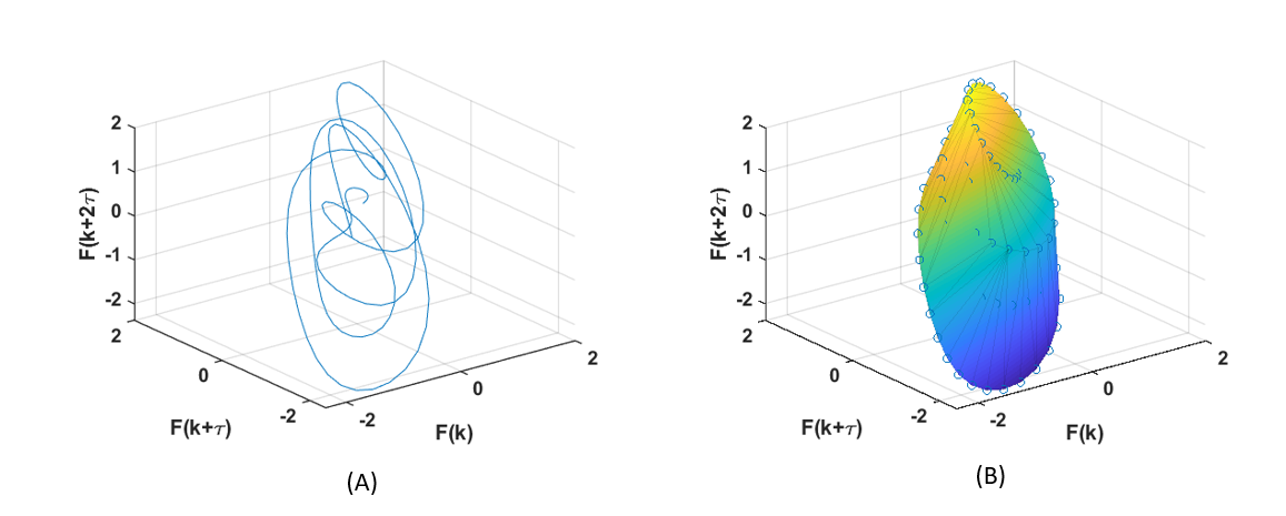
The feature we utilized in the reconstructed phase space is the sum of the length of the portrait edges (SE) 3. It is an index of the perimeter of the area of the attractor and can capture the dynamic properties of the BOLD signal, more specifically the temporal stability of the signal. An example of a BOLD signal attractor and its fitted convex hull are shown in Fig.1.
Statistical parametric maps were derived by performing voxelwise t-test of SEs between patients (SZ or ASD) and HC subjects. Statistical results were corrected for multiple comparisons using FSL tfce.4 The overview of the processing is summarized in Fig.2.
Datasets
Two schizophrenia datasets were used in the study. The first one is from the Center for Biomedical Research Excellence (COBRE).5 It consists of 64 SZ subjects (Age: 35.12 (11.58); Sex (F/M: 19/45)) and 64 healthy control (HC) subjects (Age: 37.34 (15.61); Sex (F/M: 14/50)). TR is 2s. The second one was from the Bipolar & Schizophrenia Consortium for Parsing Intermediate Phenotypes study (B-snip).6 We selected subjects with TR = 2s, resulting a dataset of 55 SZ subjects (Age: 35.20 (13.55); Sex (F/M: 28/27)) and 55 HC subjects (Age: 43.40 (11.42); Sex (F/M: 28/27)). In addition, two autism data sites, i.e., USM and UM, from the Autism Imaging Data Exchange I (ABIDE I)7 were included in this analysis. USM consists of 43 ASD subjects (Age: 22.17 (6.86); Sex (F/M: 36/7)) and 43 HC subjects (Age: 21.36 (7.64); Sex (F/M: 26/17)) with TR = 2s. UM contains 66 ASD subjects (Age: 13.17 (2.40); Sex (F/M: 57/9)) and 66 HC subjects (Age: 14.72(3.82); Sex (F/M: 48/18)). Standard prepossessing, including despiking, slice time correction, motion correction, normalization, filtering (slow-4 band: 0.027–0.073 Hz), and smoothing, was performed on the fMRI data using FSL.
Results
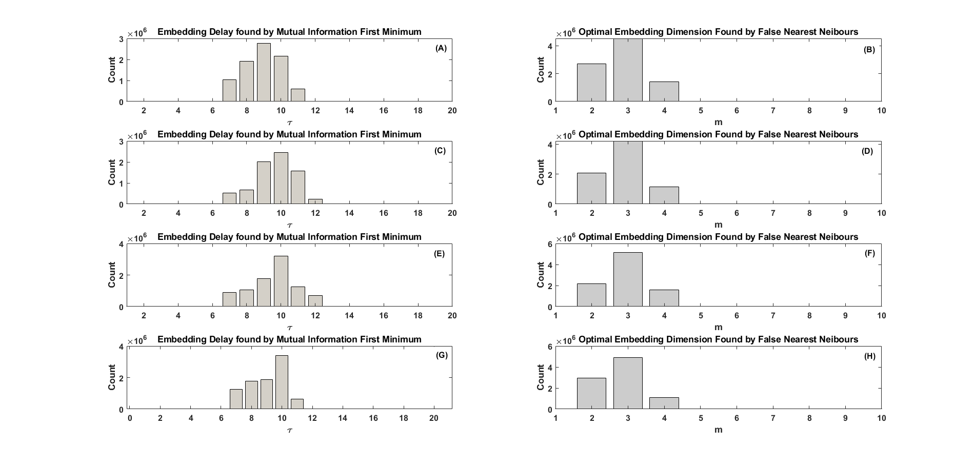
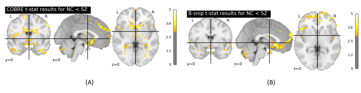
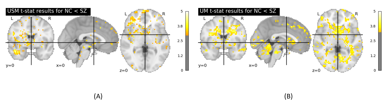
Fig.3 illustrates the histogram of choices of model parameters for the two SZ datasets and two ABIDE I datasets. The total number for each histogram is $$$N_v \times N_s$$$, where the total number of voxels of a subject $$$N_v=67749$$$, and $$$N_s$$$ is the total number of subjects of the related dataset. For the COBRE dataset, the optimal model parameters were found to be: $$$\tau=9$$$ and $$$m=3$$$. For the B-SNIP dataset, the optimal parameters were: $$$\tau=10$$$ and $$$m=3$$$. For the two ABIDE I datasets, the optimal parameters were the same, i.e., $$$\tau=10$$$ and $$$m=3$$$.The t-stat maps for SE comparison between patients and HC subjects are shown in Fig.4 (SZ) and Fig.5 (ASD), respectively. Independent t-test showed a significant increase in SE (p<0.05) in the frontal pole and subcallosal cortex regions in SZ patients compared to HC subjects for both SZ data sets. In addition, we also observed a significant SE increase (p<0.05) in the frontal pole and precentral gyrus regions in ASD subjects compared to HC subjects for both the USM and UM datasets. Our findings are consistent with previous literature.8, 9, 10, 11
Discussion and Conclusion
This paper investigated the brain dynamics of fMRI data using phase-space embedding. After the reconstruction of the phase portrait, we characterized it with the sum of the length of the edges of the convex hull, a measure capturing the dynamic stability of fMRI BOLD time courses. We applied the method to two mental disorders: SZ and ASD. The results suggest that this feature can serve as a useful marker of brain dynamics in fMRI data.Acknowledgements
We thank our colleagues from Dr.Xiaoping Hu's lab who provided insight and expertise that greatly assisted the research.References
1 N. H. Packard, J. P. Crutchfield, J. D. Farmer, and R. S. Shaw, “Geometry from a time series,” Physical review letters, vol. 45, no. 9, p. 712, 1980.
2 L. Cao, “Practical method for determining the minimum embedding dimension of a scalar time series,” Physica D: Nonlinear Phenomena, vol. 110, no.1-2, pp. 43–50, 1997.
3 M. Fedotenkova, “Mathematical modeling of level of anaesthesia from EEG measurements,” 2013.
4 S. M. Smith and T. E. Nichols, “Threshold-free cluster enhancement: addressing problems of smoothing, threshold dependence and localisation in cluster inference,” Neuroimage, vol. 44, no. 1, pp. 83–98, 2009.
5 M. S. Cetin, F. Christensen, C. C. Abbott, J. M. Stephen, A. R. Mayer, J. M.Ca ̃nive, J. R. Bustillo, G. D. Pearlson, and V. D. Calhoun, “Thalamus and posterior temporal lobe show greater inter-network connectivity at rest and across sensory paradigms in schizophrenia,” Neuroimage, vol. 97, pp. 117–126, 2014.
6 T.I.Murphy, https://ndar.nih.gov/editcollection.html?id= 2274.
7 A. Di Martino, C.-G. Yan, Q. Li, E. Denio, F. X. Castellanos, K. Alaerts, J. S.Anderson, M. Assaf, S. Y. Bookheimer and M. Daprettoet. “The autism brain imaging data exchange: towards a large-scale evaluation of the intrinsic brain architecture in autism,” Molecular psychiatry, vol. 19, no. 6, pp. 659–667, 2014.
8 P. Adamczyk, M. Wyczesany, A. Domagalik, A. Daren, K. Cepuch, P. Bładzi ́nski,A. Cechnicki, and T. Marek, “Neural circuit of verbal humor comprehension in schizophrenia-an fmri study,” NeuroImage: Clinical, vol. 15, pp. 525–540, 2017.
9 G. Mingoia, G. Wagner, K. Langbein, R. Maitra, S. Smesny, M. Dietzek, H. P.Burmeister, J. R. Reichenbach, R. G. Schl ̈osser, C. Gaseret, “Default mode network activity in schizophrenia studied at resting state using probabilistic ica,” Schizophrenia research, vol. 138, no. 2-3, pp. 143–149, 2012.
10 F.-M. Fan, H. Xiang, Y. Wen, Y.-L. Zhao, X.-L. Zhu, Y.-H. Wang, F.-D. Yang, Y.-L. Tan, and S.-P. Tan, “Brain abnormalities in different phases of working memory in schizophrenia: An integrative multi-modal MRI study,” The Journal of nervous and mental disease, vol. 207, no. 9, pp. 760–767, 2019.
11 L. Borras-Ferr ́ıs, ́U. P ́erez-Ram ́ırez, and D. Moratal, “Link-level functional connectivity neuro alterations in autism spectrum disorder: A developmental resting-state fMRI study,” Diagnostics, vol. 9, no. 1, p. 32, 2019.
Figures