3130
Predicting the temporal dynamics of the hemodynamic response using the spectrum of resting state fMRI signals
Sydney Bailes1 and Laura D. Lewis1
1Biomedical Engineering, Boston University, Boston, MA, United States
1Biomedical Engineering, Boston University, Boston, MA, United States
Synopsis
Given the substantial variations in the shape and timing of the hemodynamic response function (HRF) across the brain, it is critical to develop methods to characterize these variations for proper interpretation of the BOLD fMRI signal. Here, we identified significant differences in spectral properties of resting state fMRI signals between voxels with fast and slow hemodynamics. We found that these spectral properties can be used to classify fast and slow voxels, suggesting that information from the resting state can provide a way to understand and predict the temporal dynamics of the HRF across the brain.
Introduction
Both the shape and timing of the hemodynamic response function (HRF) vary substantially across the brain1,2, and proper characterization of these variations is critical for the interpretation of the BOLD signal obtained from fMRI3. Additionally, as techniques for fast acquisition of fMRI have become more prevalent4, the ability to assess differences in the HRF across the brain becomes even more critical5 in order to determine whether fMRI timing differences result from neural or vascular origins. Previous work has implemented breath hold6 or visual stimulus tasks7 to estimate voxel-wise differences in vascular latencies; however, these methods require additional scanning which can be difficult for certain studies or populations. We aimed to test if we can use information from the spectrum of resting state fMRI to characterize vascular delays across the brain. Since resting state scans are acquired in most studies and require no task performance on the part of the subject, using information from the resting state spectrum would provide a simple and effective way of understanding the temporal dynamics of the HRF across different regions of the brain.Methods
First, we performed simulations to determine if different temporal properties of the HRF would result in different properties of the spectrum of a voxel’s response to an identical stimulus. Six different HRFs (Fig. 1a) were defined each with a different time-to-peak (TTP), full width at half maximum (FWHM), and peak percent signal change. These properties were drawn from previous work characterizing varying HRF temporal dynamics7. We calculated the predicted fMRI response to neural activity at various frequencies by convolving oscillating stimuli (ranging 0.1-0.5 Hz) with the six defined HRFs. We also calculated the spectrum of the HRF itself.Three subjects were scanned on a 7T Siemens scanner across eight sessions, each consisting of resting state runs and runs with a flickering checkerboard visual stimulus with oscillating luminance contrast (frequency ranging 0.025-0.2 Hz, Fig. 2a-b). Functional runs consisted of 15 oblique slices positioned to include primary visual cortex (V1) acquired as single-shot gradient-echo blipped-CAIPI SMS-EPI8 with 2 mm isotropic resolution (R=2 acceleration, MultiBand factor=3, matrix=120×120, CAIPI shift=FOV/3, TR=227 ms, TE=24 ms, echo-spacing=0.59 ms, flip angle=30°). We identified voxels in V1 that were significantly driven by the stimulus using a functional localizer run and then calculated the phase delay of the response for each voxel using the arctangent of the sine and cosine regressor estimates. Then, we examined the resting state spectra of these voxels. In particular, we looked at the slope of the spectrum under 0.2 Hz, the average power under 0.1 Hz, and the exponent of the aperiodic fit (Fig. 3a). We trained k-nearest neighbors (KNN) models (N=200, 5-fold cross validation) within and across subjects to classify voxels based on these spectral properties. For the across subject model, the predictors were normalized by the mean of all voxels.
Results
Examining the simulated resting state spectra, we found that HRFs with faster dynamics exhibited less power in the low frequency bands compared to slower HRFs, but a shallow decline at higher frequencies (Fig. 1b). The slower HRFs had larger response amplitudes to lower stimulus frequencies and steeper drop-off as the stimulus frequency increased. This difference is most prominent under 0.2 Hz, after which the faster HRFs tend to have larger response amplitudes (Fig. 1c).We next identified V1 voxels as fast or slow based on their responses to the oscillating visual stimulus (Fig. 2). Each feature of the resting state spectra showed significant differences between fast and slow voxels (Wilcoxon rank sum test, ): the slopes for all 8/8 sessions and both power and aperiodic exponent for 7/8 sessions (one session had for power and for exponent) (Fig. 3b-d). We then tested whether these spectral features could predict local hemodynamic delays. We trained a KNN classifier with N=200 to identify fast and slow voxels within each subject and achieved accuracies of 78.5%, 67.1%, and 55.96%. After normalizing each metric across subjects and retraining a KNN classifier we were able to achieve a classification accuracy of 71.5%.
Discussion
Our simulation results clearly show that differences in the temporal dynamics of the HRF will change the frequency content of the fMRI response. Specifically, slower HRFs dynamics had larger response amplitudes in the low frequency band but the response quickly attenuates at higher frequencies. Conversely, faster HRFs had smaller response amplitudes in the low frequency band and a shallower slope. Notably, these differences predicted by simulations are also reflected in the resting state data: resting-state spectral features were found to be significantly different for voxels with fast versus slow hemodynamics. This allowed us to classify voxels as fast or slow both within and across subjects.Conclusion
Our results demonstrate that temporal properties of the HRF affect the spectral features of spontaneous fMRI signals. We find that this insight enables us to distinguish voxels that exhibit faster or slower hemodynamic responses using only resting state information. This finding can allow researchers to better understand the temporal properties of the HRF across voxels, which is crucial for accurate fMRI analyses, especially as we investigate faster neural dynamics.Acknowledgements
This work was funded by the NIH Grant R00-MH111748 and the NIGMS Training Program 5 T32 GM008764-20.References
- Aguirre, G. K., Zarahn, E. & D’Esposito, M. The Variability of Human, BOLD Hemodynamic Responses. NeuroImage 8, 360–369 (1998).
- de Zwart, J. A. et al. Temporal dynamics of the BOLD fMRI impulse response. NeuroImage 24, 667–677 (2005).
- Handwerker, D. A., Ollinger, J. M. & D’Esposito, M. Variation of BOLD hemodynamic responses across subjects and brain regions and their effects on statistical analyses. NeuroImage 21, 1639–1651 (2004).
- Feinberg, D. A. & Setsompop, K. Ultra-fast MRI of the human brain with simultaneous multi-slice imaging. J. Magn. Reson. San Diego Calif 1997 229, 90–100 (2013).
- Lewis, L. D., Setsompop, K., Rosen, B. R. & Polimeni, J. R. Stimulus-dependent hemodynamic response timing across the human subcortical-cortical visual pathway identified through high spatiotemporal resolution 7T fMRI. NeuroImage 181, 279–291 (2018).
- Chang, C., Thomason, M. E. & Glover, G. H. Mapping and correction of vascular hemodynamic latency in the BOLD signal. NeuroImage 43, 90–102 (2008).
- Siero, J. C. W., Petridou, N., Hoogduin, H., Luijten, P. R. & Ramsey, N. F. Cortical depth-dependent temporal dynamics of the BOLD response in the human brain. J. Cereb. Blood Flow Metab. Off. J. Int. Soc. Cereb. Blood Flow Metab. 31, 1999–2008 (2011).
- Setsompop, K. et al. Blipped-controlled aliasing in parallel imaging for simultaneous multislice echo planar imaging with reduced g-factor penalty. Magn. Reson. Med. 67, 1210–1224 (2012).
Figures
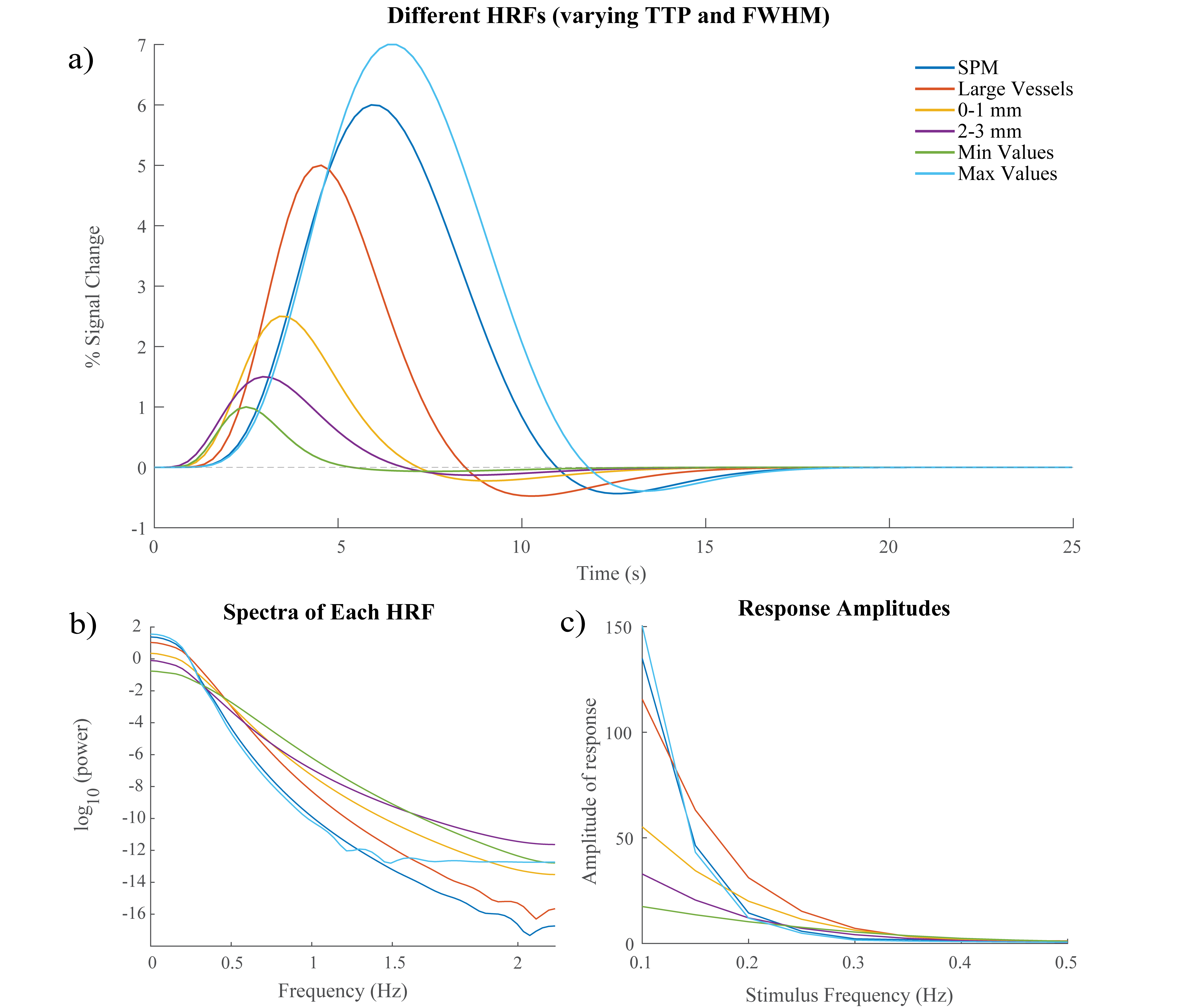
Figure 1: Simulating HRFs with
different temporal dynamics. A)
Six HRFs with varying TTPs and FWHMs that were compared in our simulation. SPM
HRF is the canonical two-gamma HRF used in SPM software while the five other
HRFs have TTPs and FWHMs based on literature7. B) Spectrum of each HRF C)
Changes in predicted fMRI response amplitude across different frequencies for
different HRF timings.
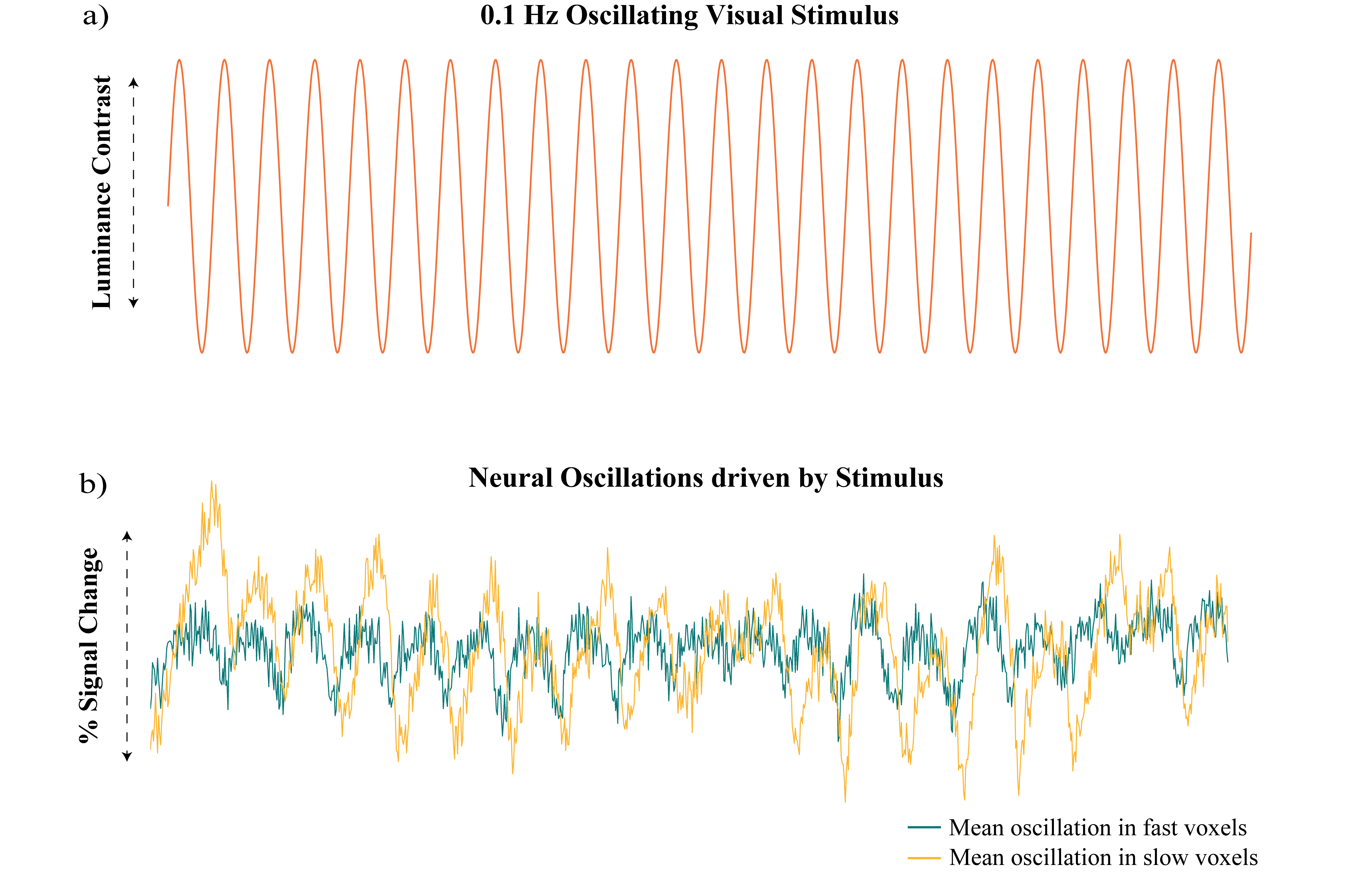
Figure 2: Visual
stimulus driving neural oscillations and selection of fast/slow voxels. A) A checkerboard with
oscillating luminance contrast (0.1 Hz) was presented to the subjects to drive
neural oscillations in V1. B) Example of mean neural oscillations in response to stimulus in slow and fast
voxels for a single subject.
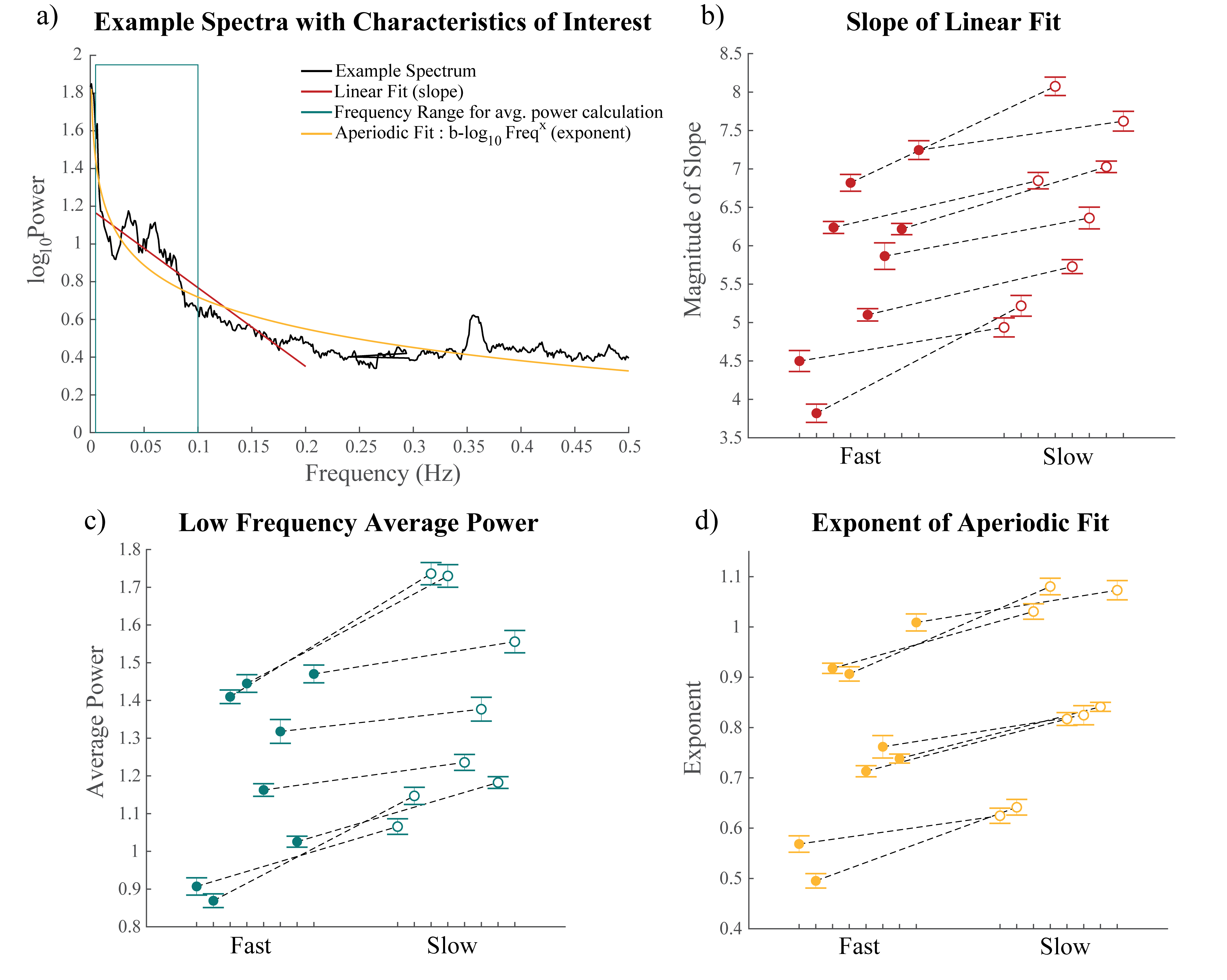
Figure 3: Differences in resting
state spectra across fast and slow voxels. A) Example spectrum showing how each variable shown in
Fig. 3b-d were calculated. B-D)
Differences in the average of the B) slopes of the resting state spectrum, C) average
power, and D) exponent of fit to b-log10Freqx fast and slow
voxels in a session, 8/8 slope, 7/8 low frequency power, 7/8 aperiodic exponent
pairings have significant difference (p<0.5), error bars report SEM.