3127
Spatiotemporal Trajectories in Resting-state FMRI Revealed by Convolutional Variational Autoencoder1BME, Emory University/Georgia Tech, Atlanta, GA, United States
Synopsis
We trained a novel convolutional variational autoencoder to extract intrinsic spatial temporal patterns from short segments of resting-state fMRI data. The network was trained in an unsupervised manner using data from the Human Connectome Project. The extracted latent dimensions not only show clear clusters in the spatial domain that were in agreement with DMN/TPN anticorrelations and principal gradients, but also provide temporal information as well. The method provides a way to extract orthogonal spatial temporal patterns within fMRI data in a short time window, among which many patterns were not previously discovered and are worth investigating in the future.
Introductions
Recent studies have shown that the human brain consists of several networks with distinct functions, and their connectivity is dynamically evolving over time. Many methods have been proposed to study the dynamic aspect of functional connectivity among these major networks, including independent component analysis (ICA), sliding window correlation (SWC), quasiperiodic patterns (QPPs), co-activation patterns (CAPs) and hidden-Markov models (HMM) [1-7]. However, Most of these methods consider spatial and temporal information separately, when in reality the temporal and spatial aspects of brain activity are intricately related. Here we proposed to train a convolutional variational autoencoder using resting-state fMRI data to identify common spatiotemporal trajectories that describe the flow of activity across the brain.Methods
FMRI data preprocessing:The minimally processed resting state and fMRI data was downloaded from the Human Connectome Project (HCP) S500 release [8]. The first 5 frames were removed to minimize the transient effects. Gray matter, white matter and cerebrospinal fluid signals, 12 motion parameters (all provided by HCP), linear and quadratic trends were regressed out altogether pixel-wisely. The regressed BOLD signals were then band pass filtered using a 0.01-0.1Hz 6-order Butterworth filter, and spatially smoothed using a Gaussian kernel (FWHM=2pixel). Finally, the BOLD signals were parcellated using Brainnetome atlas [9] and z-scored. The final parcellated BOLD signal has 412 subjects by 1195 time points (TR=0.72s) by 246 parcels. For better visualization, the 246 parcels were then sorted into 7 functional networks using Yeo’s 7-network model [10] provided by Brainnetome website, namely the default mode (DMN), visual (VIS), somatomotor (SM), dorsal attention (DA), ventral attention (VA), frontal parietal (FP), limbic (LIM) networks and subcortical regions (SC).
Convolutional Variational Autoencoder:
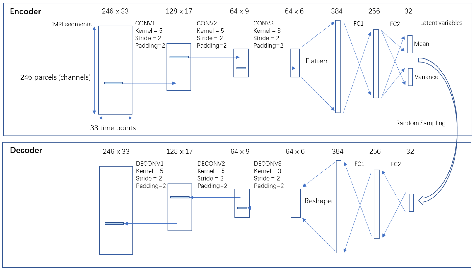
A variational autoencoder (VAE) [11] with 1-D convolutional layers applying to the temporal dimension was implemented using pytorch [12], based on the assumption that the rules governing the network dynamics are shift-invariant across time. This neural network (architecture shown in figure 1) was selected instead of a plain autoencoder because both the random sampling in variational autoencoder and the parameter sharing in the convolutional layer improve generalizability. The 412 subjects were randomly split into training set (n=248), validation set (n=82) and testing set (n=82). Each fMRI scan (1195 TR) was divided into 36 segments that are 33-TR long (23.76sec), with 50% overlapping. The 33-TR segment length was chosen based on prior work identifying a strong spatiotemporal pattern with a duration of ~20s [5]. Then the segments were shuffled, resulting a training set with size of [248x36,246,33], a validation set and a testing set both with size of [82x36,246,33]. The loss function is the sum of reconstruction loss (root mean square error between input and output) and the Kullback-Leibler (KL) divergence loss. The networks were trained on a Nvidia GTX2080Ti GPU using Adam optimizer [13] with a learning rate of 0.001 for 90 epochs.
Results and Discussions
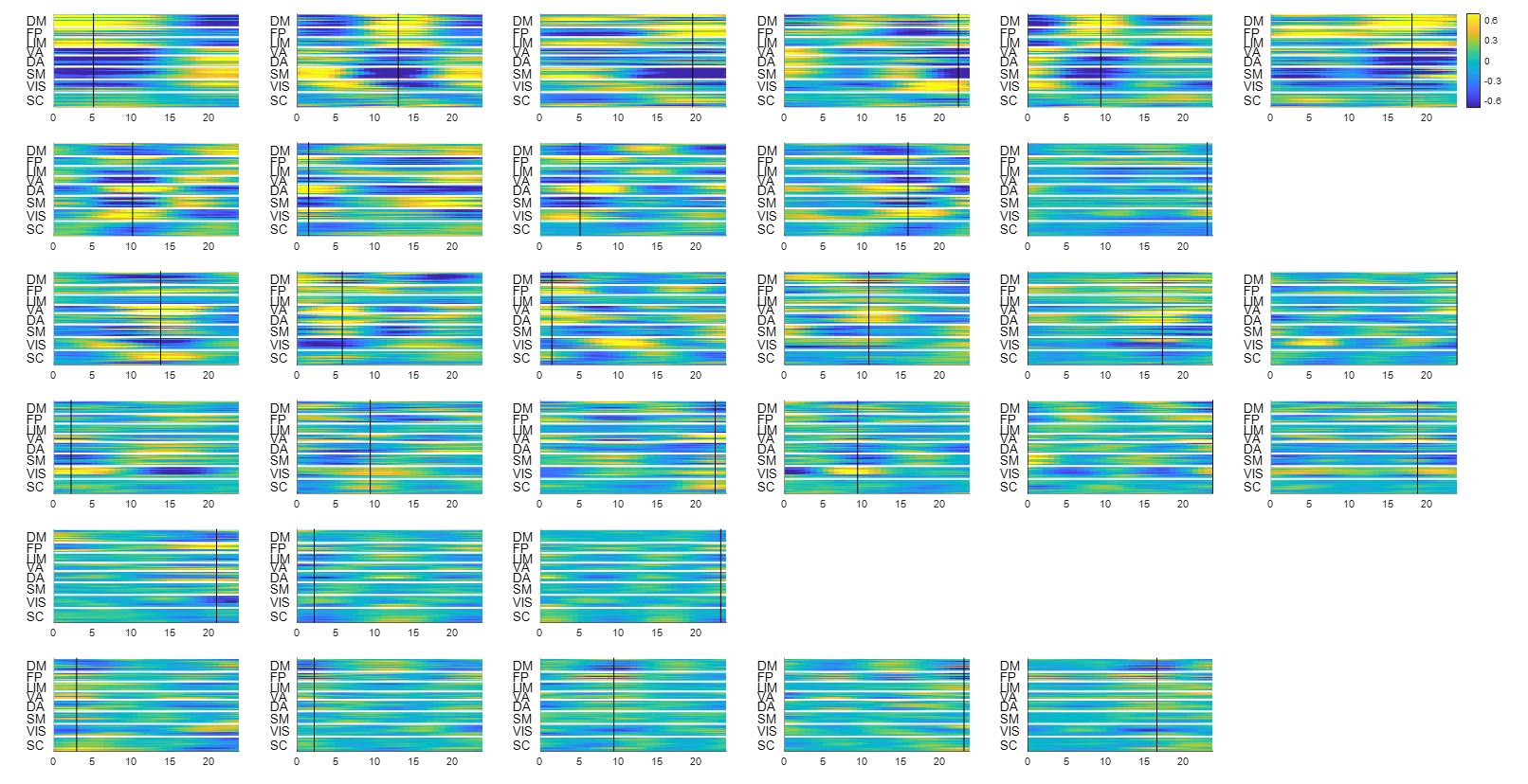
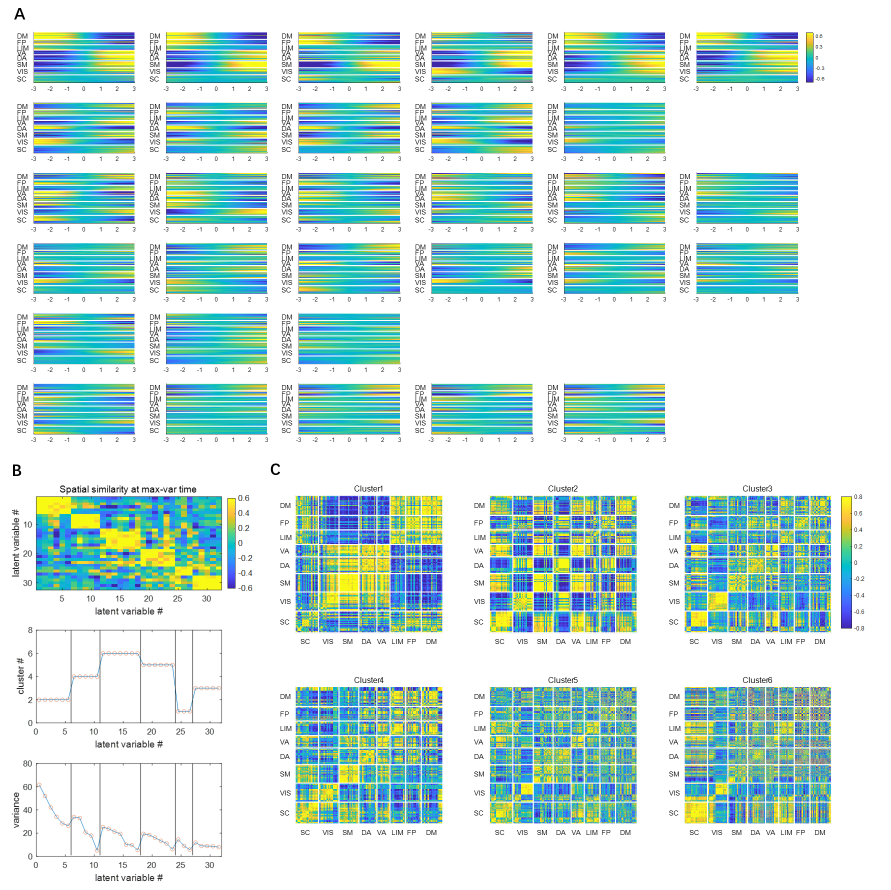
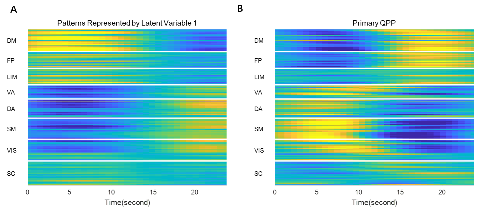
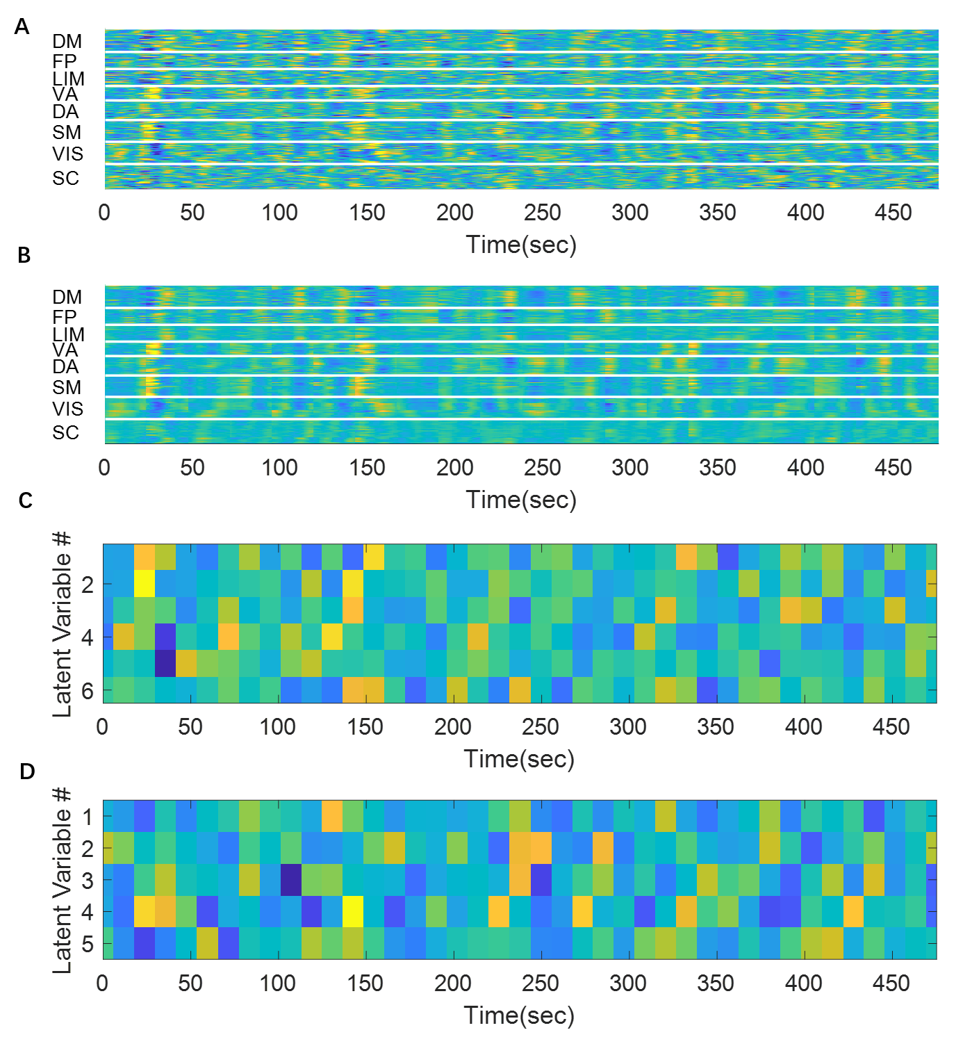
Since the latent variables should be multidimensional standard Gaussian distribution (all components are independent, zero-mean, unit-variance), which is encouraged by penalizing the KL divergence, the features extracted by the latent variables are almost orthogonal to each other. Thus the spatial temporal feature can be visualized by propagating change along individual latent dimension through the trained decoder, which is shown in Figure 2. Note that many latent variables are spatially similar to each other, thus they were further organized into several groups based on the spatial profiles at the time points when the variance across the spatial dimension reaches its maximum (shown as black cursors in figure 2). The latent variables were grouped into 6 spatially similar clusters using K-means clustering method, and were sorted by their variance explained, as illustrated in figure 3.It can be seen that within the primary cluster, whose mean variance is the highest, every latent dimension has the DMN and FPN on one end, whereas the task positive network (TPN), which includes VIS, SM, DA, VA, is on the opposite end. This finding agrees with many previous studies, including the DMN/TPN anticorrelation found in [14] and QPPs [5]. The secondary cluster further separates different networks within the TPN, by having VIS and DA on one end and SM and VA on the other end. This together with the primary cluster share remarkably high resemblance with principal gradient 1 and 2 [15]. In addition, the feature learned by the first latent dimension is very similar to the primary QPP as well (shown in figure 4). But VAE also offers many other spatial temporal features that have different frequencies, which were not previously discovered by QPP, whose role in brain function is worth further investigating. Figure 5 shows the reconstruction of the signal and the corresponding weights of latent variables, which provide a compact representation of brain activity.
Conclusion
In this abstract we proposed a novel convolutional variational autoencoder to extract intrinsic spatial temporal patterns from short segments of resting-state fMRI data. The extracted latent dimensions show clear clusters in the spatial domain that were in agreement with previous findings, but also provide temporal information as well. Some spatial temporal features were similar to QPPs, but there are others with smaller variances that were not previously discovered, which is worth investigating in the future.Acknowledgements
Funding sources: NIH 1 R01NS078095-01, BRAIN initiative R01 MH 111416 and NSF INSPIRE. The authors would like to thank the Washington University–University of Minnesota Consortium of the Human Connectome Project (WU-Minn HCP) for generating and making publicly available the HCP data. The authors would like to thank Chinese Scholarship Council (CSC) for financial support.References
1. Beckmann CF, Smith SM. Probabilistic independent component analysis for functional magnetic resonance imaging. IEEE transactions on medical imaging. 2004 Feb 6;23(2):137-52.
2. Calhoun VD, Adali T, Pearlson GD, Pekar JJ. A method for making group inferences from functional MRI data using independent component analysis. Human brain mapping. 2001 Nov;14(3):140-51.
3. Allen EA, Damaraju E, Plis SM, Erhardt EB, Eichele T, Calhoun VD. Tracking whole-brain connectivity dynamics in the resting state. Cerebral cortex. 2014 Mar 1;24(3):663-76.
4. Chang C, Glover GH. Time–frequency dynamics of resting-state brain connectivity measured with fMRI. Neuroimage. 2010 Mar 1;50(1):81-98.
5. Majeed W, Magnuson M, Hasenkamp W, Schwarb H, Schumacher EH, Barsalou L, Keilholz SD. Spatiotemporal dynamics of low frequency BOLD fluctuations in rats and humans. Neuroimage. 2011 Jan 15;54(2):1140-50.
6. Liu X, Duyn JH. Time-varying functional network information extracted from brief instances of spontaneous brain activity. Proceedings of the National Academy of Sciences. 2013 Mar 12;110(11):4392-7.
7. Vidaurre D, Smith SM, Woolrich MW. Brain network dynamics are hierarchically organized in time. Proceedings of the National Academy of Sciences. 2017 Nov 28;114(48):12827-32.
8. Glasser MF, Sotiropoulos SN, Wilson JA, Coalson TS, Fischl B, Andersson JL, Xu J, Jbabdi S, Webster M, Polimeni JR, Van Essen DC. The minimal preprocessing pipelines for the Human Connectome Project. Neuroimage. 2013 Oct 15;80:105-24.
9. Fan L, Li H, Zhuo J, Zhang Y, Wang J, Chen L, Yang Z, Chu C, Xie S, Laird AR, Fox PT. The human brainnetome atlas: a new brain atlas based on connectional architecture. Cerebral cortex. 2016 Aug 1;26(8):3508-26.
10. Yeo BT, Krienen FM, Sepulcre J, Sabuncu MR, Lashkari D, Hollinshead M, Roffman JL, Smoller JW, Zöllei L, Polimeni JR, Fischl B. The organization of the human cerebral cortex estimated by intrinsic functional connectivity. Journal of neurophysiology. 2011 Sep 1.
11. Kingma DP, Welling M. Auto-encoding variational bayes. arXiv preprint arXiv:1312.6114. 2013 Dec 20.
12. Paszke A, Gross S, Chintala S, Chanan G, Yang E, DeVito Z, Lin Z, Desmaison A, Antiga L, Lerer A. Automatic differentiation in pytorch.
13. Kingma DP, Ba J. Adam: A method for stochastic optimization. arXiv preprint arXiv:1412.6980. 2014 Dec 22. Glasser MF, Sotiropoulos SN, Wilson JA, Coalson TS, Fischl B, Andersson JL, Xu J, Jbabdi S, Webster M, Polimeni JR, Van Essen DC. The minimal preprocessing pipelines for the Human Connectome Project. Neuroimage. 2013 Oct 15;80:105-24.
14. Fox MD, Snyder AZ, Vincent JL, Corbetta M, Van Essen DC, Raichle ME. The human brain is intrinsically organized into dynamic, anticorrelated functional networks. Proceedings of the National Academy of Sciences. 2005 Jul 5;102(27):9673-8.
15. Margulies DS, Ghosh SS, Goulas A, Falkiewicz M, Huntenburg JM, Langs G, Bezgin G, Eickhoff SB, Castellanos FX, Petrides M, Jefferies E. Situating the default-mode network along a principal gradient of macroscale cortical organization. Proceedings of the National Academy of Sciences. 2016 Nov 1;113(44):12574-9.
Figures