3126
Evaluation of spatial blur induced by preprocessing and distortion in UHF fMRI data1Department of Neurology of the Second Affiliated Hospital, Interdisciplinary Institute of Neuroscience and Technology, School of Medicine, Zhejiang University, Hangzhou, China, 2Athinoula A. Martinos Center for Biomedical Imaging, Massachusetts General Hospital, Charlestown, MA, United States, 3Department of Radiology, Harvard Medical School, Charlestown, MA, United States, 4Key Laboratory for Biomedical Engineering, of Ministry of Education, Zhejiang University, Hangzhou, China, 5Division of Health Sciences and Technology, Massachusetts Institute of Technology, Cambridge, MA, United States
Synopsis
Functional MRI is vulnerable to several sources of spatially-varying blurring imposed both at the data acquisition and analysis stages. For studies investigating fine-scale functional organization, any losses in imaging resolution, caused by blurring, dramatically affect the interpretation of the data. Therefore, these often-unavoidable blurring effects should be taken into account. Here we suggest approaches to minimize losses in spatial accuracy and recommend methods for quantifying the imaging resolution. These quantification methods can provide spatial “error bars” to use when evaluating results.
Introduction
Ultra-High Field (≥7T) functional Magnetic Resonance Imaging (UHF-MRI) provides opportunities to resolve fine-scale features of functional architecture like cortical columns1–4 and layers5–7 in vivo. These relevant features are, however, at the edge of the imaging resolution that can be achieved with modern fMRI technologies8. While the nominal resolution of our acquisitions may appear to be sufficient to resolve these features, there are many well-known sources of unwanted spatial blurring, such as T2* decay in EPI, that result in losses of effective imaging resolution9,10, which impede our ability to detect these features. What is less well appreciated is that data processing will also cause unavoidable losses in effective resolution11,12. Here we consider additional sources of blurring imposed both at the data acquisition and analysis stages, including resolution losses due to projecting fMRI data on to cortical surface reconstructions and the losses (and potential gains) in resolution associated with geometric distortion. We suggest several approaches to minimize losses in spatial accuracy and to quantify the imaging resolution. These quantification methods enable principled comparisons between preprocessing strategies and provide spatial “error bars” to use when evaluating results.Methods
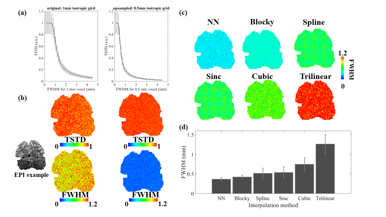
Three healthy volunteers, after providing written informed consent, participated in the study. Data were acquired on a whole-body 7 Tesla scanner (Siemens MAGENTOM). Functional MRI data were acquired with a nominally 1-mm isotropic single-shot gradient-echo EPI protocol. Details of sequence parameters and V2 stripes detection paradigm can be found in Nasr et al. (2016)2.To quantify/compare the level of spatial blurring induced during preprocessing, we followed a procedure employed previously12,13 based on generating a synthetic i.i.d. white-noise time series on 1-mm isotropic grid matching that of the functional data, and subjecting this 4D noise volumes to various preprocessing steps. We numerically determined the mapping between temporal standard deviation (TSTD) and resolution losses by applying 3D gaussian smoothing kernels to the original 4D noise data with varying smoothing capacity.
Using this approach, we compared the implicit smoothing imposed by different processing strategies. Specifically, we evaluated (1) the influence of sequential interpolation steps versus a one-step resampling; (2) the influence of upsampling the voxel grid prior to these interpolation steps; (3) the effects of different interpolation algorithms; (4) the effects of upsampling the triangular mesh that comprises the cortical surface model.
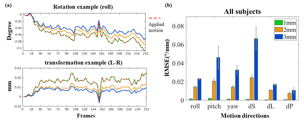
Because mis-estimated motion will also result in loss of spatial accuracy imposed by motion correction, we also quantified the influence of imaging resolution on motion parameter estimation accuracy. This was achieved by synthesizing a 4D volume with known motion through applying realistic motion trace (generated from the motion estimation of similar fMRI data), then down-sampling this synthetic 4D volume to achieve larger voxel sizes. The motion of three 4D volumes was estimated, at different voxel sizes, using the AFNI tool 3dvolreg. The motion estimation error was then calculated between the parameters of true (applied) and estimated motion for each voxel size.
Finally, we provided an example of how true imaging resolution can vary due to geometric distortion, which not only displaces voxels but also can expand or compress voxel sizes, leading to another form of spatially-varying resolution across brain regions. We evaluated the voxel compression/expansion imparted by several gradient coil sets by simply computing the Jacobian determinant of the deformation induced by gradient nonlinearity.
Results
The results of Fig. 1b demonstrate upsampling can substantially reduce the blurring effects of interpolation (during motion correction). Figs. 1c & d demonstrate the blurring imposed by several interpolation methods; while the results largely conform to expectations, the ‘blocky’ interpolation method (as implemented in AFNI) appears to outperform higher-order interpolation methods such as spline and cubic.Fig. 2 shows the error of motion estimation decreases as image resolution increases. While higher-resolution data are more likely to be corrupted by small motion, this result suggests that the smaller voxels may partly compensate for this effect.
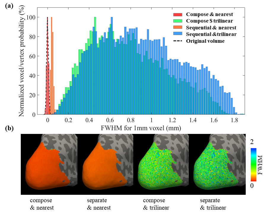
Fig. 3 demonstrates that composing two transformations has a relatively small effect on the final resolution, however if more transformations were to be employed the benefits of composing are expected to increase.
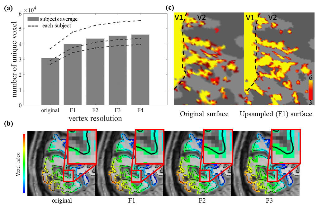
The effects of surface mesh upsampling on data quality are shown in Fig. 4, where the finer meshes not only capture more unique fMRI voxels but they also provide more details of the V2 stripe columnar pattern that agree better with our expectations based on classic histology studies.
Fig. 5 demonstrate how the geometric distortions impart a spatially-varying resolution modulation, and this pattern changes for each gradient coil due to their differences in gradient nonlinearity.
Discussion
This study suggests methods to evaluate spatial blur in fMRI data. We showed that, not only is the level of data blurring dependent on analysis choices, but it is non-uniform over the brain. The formulation of hypotheses and the interpretation of the results should take into account the final spatial resolution. We therefore recommend generating spatial resolution maps alongside activation maps to account for the spatially-varying resolution. In future work we will consider the impact of these effects on statistical inference and multiple comparisons correction14,15. We note that we have previously evaluated aspects of the image reconstruction, such as partial Fourier, that also influence the final imaging resolution16, were not considered here.Acknowledgements
We thank Mr. Kyle Droppa for his assistance with human participant scanning. This work was supported in part by a 2019 Zhejiang University Academic Award for Outstanding Doctoral Candidates (2019075), the program of China Scholarships Council (201906320397), the grant from National Key R&D Program of China 2018YFA0701400, the National Natural Science Foundation of China (8191101288, 31627802), the key research and development program of Zhejiang province 2020C03004, the Fundamental Research Funds for the Central Universities (2019XZZX003-20), the NIH NIBIB (grants P41-EB030006 and R01-EB019437), NIH NIMH (grant R01-MH124004), by the BRAIN Initiative (NIH NIMH grant R01-MH111419), the NIH NEI (R01EY026881 and R01EY030434), by the MGH/HST Athinoula A. Martinos Center for Biomedical Imaging; and was made possible by the resources provided by NIH Shared Instrumentation Grant S10-RR019371.References
1. Cheng K, Waggoner RA, Tanaka K. Human Ocular Dominance Columns as Revealed by High-Field Functional Magnetic Resonance Imaging. Neuron. 2001;32(2):359-374.
2. Nasr S, Polimeni JR, Tootell RBH. Interdigitated Color- and Disparity-Selective Columns within Human Visual Cortical Areas V2 and V3. Journal of Neuroscience. 2016;36(6):1841-1857.
3. Yacoub E, Shmuel A, Logothetis N, Uğurbil K. Robust detection of ocular dominance columns in humans using Hahn Spin Echo BOLD functional MRI at 7 Tesla. NeuroImage. 2007;37(4):1161-1177.
4. Yacoub E, Harel N, Uğurbil K. High-field fMRI unveils orientation columns in humans. Proceedings of the National Academy of Sciences. 2008;105(30):10607–10612.
5. Muckli L, De Martino F, Vizioli L, et al. Contextual Feedback to Superficial Layers of V1. Current Biology. 2015;25(20):2690-2695.
6. Huber L, Handwerker DA, Jangraw DC, et al. High-Resolution CBV-fMRI Allows Mapping of Laminar Activity and Connectivity of Cortical Input and Output in Human M1. Neuron. 2017;96(6):1253-1263.e7.
7. Norris DG, Polimeni JR. Laminar (f)MRI: A short history and future prospects. NeuroImage. 2019;197:643-649.
8. Polimeni JR, Wald LL. Magnetic Resonance Imaging technology — bridging the gap between noninvasive human imaging and optical microscopy. Current Opinion in Neurobiology. 2018;50:250-260.
9. Chaimow D, Shmuel A. A More Accurate Account of the Effect of K-Space Sampling and Signal Decay on the Effective Spatial Resolution in Functional MRI. Neuroscience; 2016.
10. Farzaneh F, Riederer SJ, Pelc NJ. Analysis of T2 limitations and off-resonance effects on spatial resolution and artifacts in echo-planar imaging. Magn Reson Med. 1990;14(1):123-139.
11. Glasser MF, Sotiropoulos SN, Wilson JA, et al. The minimal preprocessing pipelines for the Human Connectome Project. NeuroImage. 2013;80:105-124.
12. Polimeni JR, Renvall V, Zaretskaya N, Fischl B. Analysis strategies for high-resolution UHF-fMRI data. NeuroImage. Published online April 2017.
13. Renvall V, Witzel T, Wald LL, Polimeni JR. Automatic cortical surface reconstruction of high-resolution T1 echo planar imaging data. NeuroImage. 2016;134:338-354.
14. Eklund A, Nichols TE, Knutsson H. Cluster failure: Why fMRI inferences for spatial extent have inflated false-positive rates. Proc Natl Acad Sci USA. 2016;113(28):7900-7905.
15. Wald LL, Polimeni JR. Impacting the effect of fMRI noise through hardware and acquisition choices – Implications for controlling false positive rates. NeuroImage. 2017;154:15-22.
16. Zaretskaya N, Polimeni JR. Partial Fourier imaging anisotropically reduces spatial independence of BOLD signal time courses. Present 22nd Annu Meet Organ Hum Brain Mapping, June 26--30, 2016, Geneva, Switz. 2016;22.
Figures