3116
Automatic 3D B1 field mapping using 3D printer and digital oscilloscope for gradient-free MRI system
Yonghyun Ha1, Kartiga Selvaganesan1, Sajad Hosseinnezhadian1, Baosong Wu1, Kasey Hancock1, Gigi Galiana1, and R. Todd Constable1
1Department of Radiology and Biomedical Imaging, Yale School of Medicine, New Haven, CT, United States
1Department of Radiology and Biomedical Imaging, Yale School of Medicine, New Haven, CT, United States
Synopsis
For gradient-free RF spatial encoding, MR image based B1 mapping methods cannot be used due to the absence of gradient coils. However, it is important to get a B1 map particularly if Bloch-Siegert shift encoding is used. In this work, a method to automatically measure the amplitude of B1 field is introduced. Three perpendicular pickup loops were used to measure the B1 field in three orthogonal axes simultaneously. The position of the pickup loops was controlled by 3D printer, and the peak-to-peak voltage of the coupled signal was automatically saved using PC oscilloscope.
Purpose
In conventional magnetic resonance imaging (MRI) system, three gradient coils are commonly used for spatial encoding1. However, fast switching of the B0 gradients involves undesired effects such as vibration, acoustic noise, eddy current, and peripheral nerve stimulation (PNS), in addtion to requiring significant hardware and intorducing design constrints on openness. One method to avoid these negative effects is using RF gradients2,3 for spatiaal encoding, and approach that is especially suitable for low-field applications, where SAR is less problematic. To reconstruct images encoded by RF, the RF magnetic field (B1) must be known across the entire imaging volume. The B1 map is often measured using MR images on conventional MR systems4 but these methods cannot be used on an MR systems lacking gradient coils. Thus, another way to measure the B1 map is required for imaging using RF for spatial encoding. The purpose of this work is to measure the B1 map automatically using a 3D printer and oscilloscope.Methods
To measure the B1x, B1y, B1z simultaneously, a probe consisting of three pickup loops (square coils, copper wire on the 3D printed frame, 10mm × 10mm × 10mm) was used (Fig. 1). Each of the pickup loops is arranged perpendicular to the others, such that the directions of the magnetic fields created by the three loops are also perpendicular to each other. This configuration also means that, they do not influence the other loops (isolations between the loops were higher than 77 dB at 1 MHz). The probe was fixed at the one end of an acrylic cylinder. If the extruder module of the 3D printer moves in three dimensions, fixing the acrylic cylinder to the extruder module should be sufficient to control the position of the probe. However, many commercial 3D printers are designed such that the extruder moves in two dimensions, and the bed moves in one dimension. The 3D printer used here (Ender 3, Creality, China) also moves the extruder in the x-z direction and the bed in the y direction. Below is a detailed description of how this printer can be used for positioning of the probe. A guide for the acrylic cylinder was designed and printed using the 3D printer and this guide was fixed on the extruder module of the 3D printer. When the extruder module moves in x and/or z direction, the probe moves together but still can slide in y direction. The other end of the acrylic cylinder was fixed in a plastic holder which is also printed using the 3D printer. This plastic holder can slide along the Teflon bar in the x direction. The Teflon bar can slide in the z direction along the two guide bars which are fixed on the bed. Thus, the plastic holder slides in the x-z direction following the movement of extruder, and movement in the y-direction follows the movement of the bed. The movement of the probe was controlled by g-code which was written using Python. Three pickup loops were connected to the digital oscilloscope via co-axial cables. This oscilloscope (Picoscope 4824, Pico technology, UK) was connected to the PC, and saved peak-to-peak values for each second during the B1 field scanning. A batch file was written for this purpose. B1 magnitude in x, y, and z direction was calculated using below equation after measurement.$$B_1=\frac{V_{pp}}{2\omega A},$$where $$$V_{pp}$$$, $$$\omega$$$, and A are peak-to-peak voltage, resonance frequency, and cross-sectional area of the loop. Using this set up, the B1 field generated by circular surface coil was obtained (ROI: 110mm × 110mm × 50mm, resolution: 10mm × 10mm × 10mm, scan time: 14m 29s). Figure 3 shows the scan trajectory. The surface coil (10 mm diameter, 5 turn surface coil) was tuned at 870 kHz and placed on an open magnet. The static magnetic field was also applied during the measurement, with a field strength of 24 mT at the bottom of the magnet5.Results
Figure 4 shows the B1 map of the surface coil. The magnitudes of B1x, and B1y were large near the wire. In particular they were highest where the wire is aligned perpendicular to the magnetic field direction (x and y direction for B1y and B1x respectively). The magnitude of B1z inside of the coil was larger than that outside of the coil.Discussion
We have automatically measured the amplitude of all three components of the RF magnetic field using a 3D printer and oscilloscope. This approach is useful in developing gradient-free MR system that rely of RF Bloch-Siegert shift for spatial encoding. The design approach demonstrated here can be adapted for higher field MRI since the acrylic cylinder and 3-axis probe are non-magnetic. This system can also be adapted for measuring B0 field by replacing the 3-axis probe with a Hall effect probe. In addition, B0 and B1 field mapping could be performed simultaneously by adding the Hall probe at the center ot the three pickup loops.Conslusions
We have introduced a method to automatically measure the 3D B1 field using commercial 3D printer and oscilloscope. We demonstrated that the magnitude of the B1x, B1y, and B1z can be measured simultaneously using three perpendicular loops.Acknowledgements
No acknowledgement found.References
1. S. Hidalgo-Tobon, “Theory of gradient coil design methods for magnetic resonance imaging,” concepts Mat. Reson. Part A, vol. 36, no. 4, pp. 223-242, Jul. 2010. 2. J. C. Sharp, S.B. King, “MRI using radiofrequency magnetic field phase gradients,” Magn, Reson, Med., vol. 63, no. 1, pp. 151-161, Jan. 2010. 3. R. Kartäusch, T. Driessel, T. Kampf, T. C. Basse-Lüsebrink, and U. C. Hoelscher, “Spatial phase encoding exploiting the Bloch-Siegert shift effect,“ Magn. Reson. Mat. Phys. Bios. Med., vol. 27, no. 5, pp. 363-371, Oct. 2014. 4. L. I. Sacolick, F. Wiesinger, I. Hancu, and M. W. Vogel, „ B1 mapping by Bloch-Siegert shift,“ Magn. Reson. Med., vol. 63, no. 5, pp. 1315-1322, May 2010. 5. R. T. constable, C. Rogers III, B. Wu, K. Selvaganesan, and G. Galiana, “Design of a novel class of open MRI devices with nonuniform B0, field cycling, and RF spatial encoding,” in Proc. 27th annu. Meet. Int. Soc. Magn. Res. Med., Montreal, Canada, May 10-13, 2019.Figures
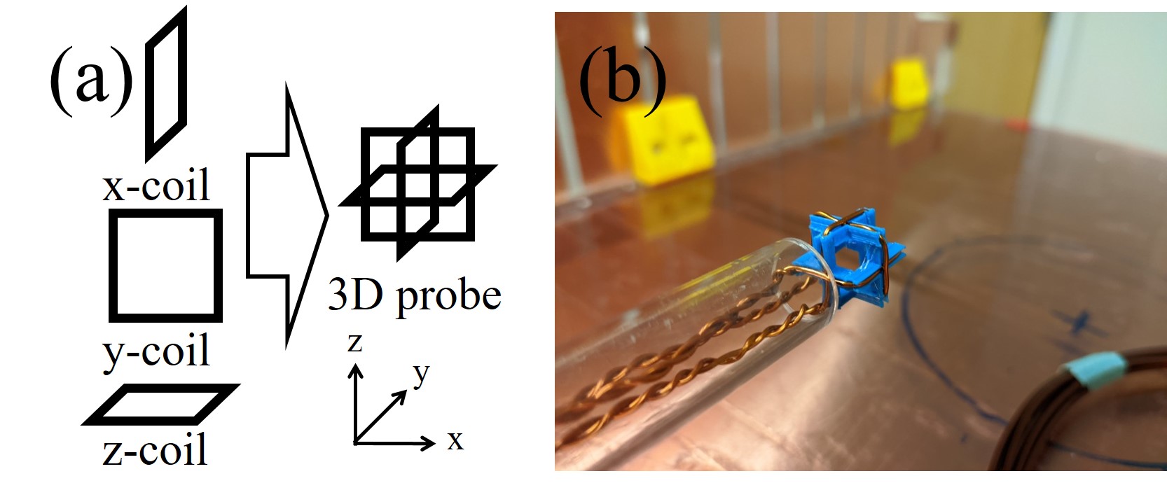
Figure 1. (a) Scheme and (b) photo of the 3-axis probe. The probe consists with three perpendicular square loops.
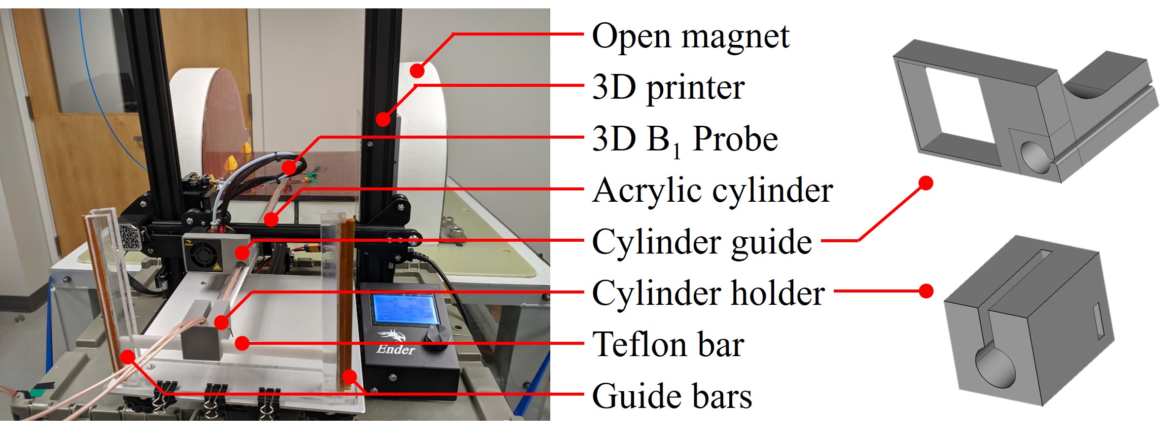
Figure 2. Experimental set up.
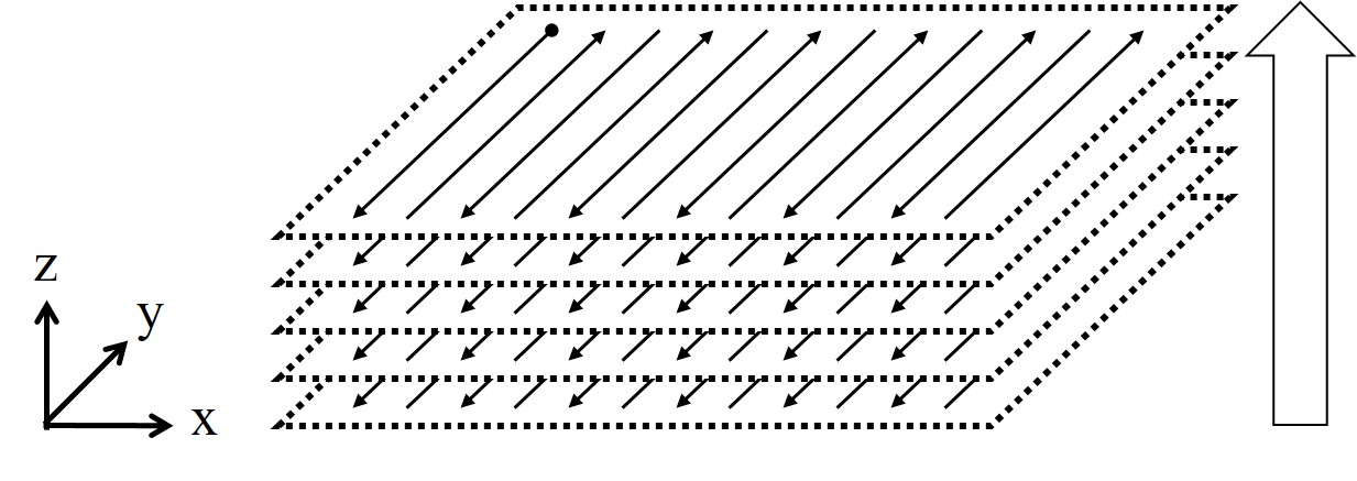
Figure 3. Measurement tajectory.
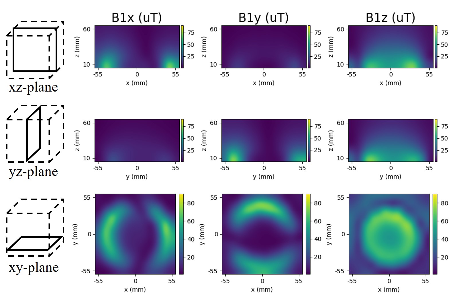
Figure 4. Measured B1x (left column), B1y (middle column), and B1z (right column) on xz-plane (sagittal, top row), yz-plane (transversal, center row), and xy-plane (coronal, bottom row). Note that, The main magnetic field direction is y-axis.