3101
Systematic, Linear Algebra-based Dimensional Analysis of Gradient Inductance Scaling with Coil Radius1Radiology, Mayo Clinic, Rochester, MN, United States, 2Biomedical Engineering, Sungkyunkwan University, Suwon, Korea, Republic of
Synopsis
Applying systematic dimensional analysis based linear algebraic methods, we derive the important scaling relation for MR gradient design: gradient coil inductance L scales as the square gradient efficiency (measured in T/m/A) and the fifth power of radius. The inclusion of "turns" as a unit in the dimensional matrix produces the result uniquely, greatly simplifying the analysis.
Introduction
An important result in gradient design is the inductance L of gradient coil scales as the fifth power of the coil’s radius a. The proportionality relationship L α a5 holds provided the primary and shield layers are sufficiently well-separated [1-2]. Coil inductance plays a central role in gradient performance because the stored energy is given by Ws = ½LI2 where I is the coil current, and gradient risetime τ=LI (V-IR) -1, where V is the applied voltage and R is the coil resistance.The scaling relationship L α a5 has had a major impact on MR gradient performance as well as power and chilled-water requirements as the standard patient aperture has increased from 60 to 70 cm, which approximately doubles inductance. Also, along with reduced peripheral nerve stimulation [3,4], the scaling of L strongly motivated for advent of smaller bore size scanners and gradient coil inserts, e.g. [5-7]. Here we examine the basis of this important scaling relationship using systematic, dimensional analysis methods that are based on linear algebra [8-9].
Methods
To apply systematic dimensional analysis we seek a set of exponents (e1,e2 … en ) such that the product of a set of n physical parameters (q1e1 × q2e2 ×...qnen) equals to 1, i.e., is dimensionless. We are free to choose the set of q based on experience or modeling, as detailed in [8-9].Consider the five physical quantities L (inductance in H), G (gradient amplitude in T/m), a (radius in m), μ0 (permeability of free space in H/m), and I (current in A). L is the quantity being investigated, and the inclusion of the other four is motivated by their appearance as dimensioned quantities in the expression for G in simple gradients for which an analytical result can be written, e.g., a Maxwell coil pair (e.g., see Eq. 6 in [10]).
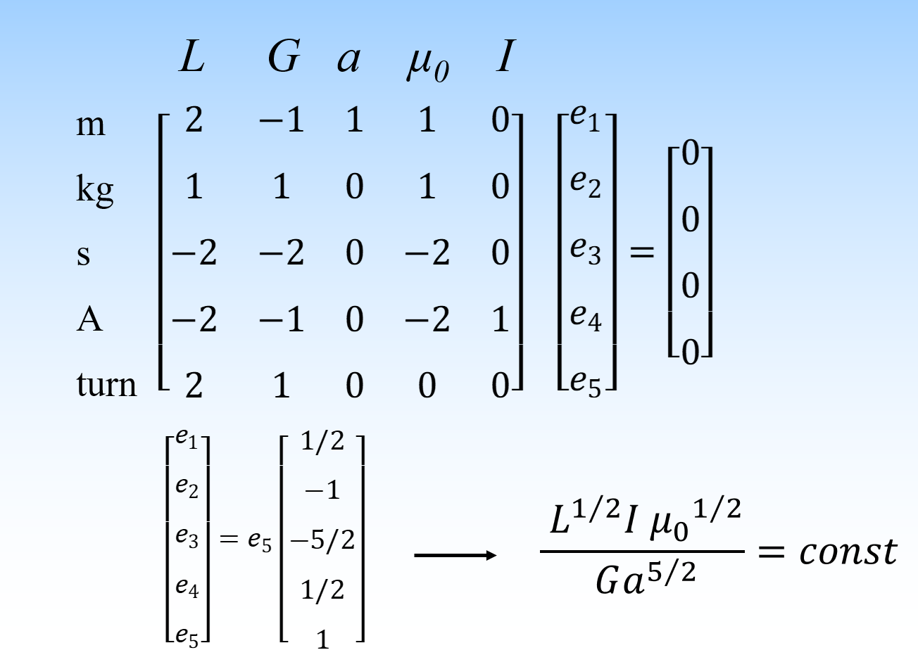
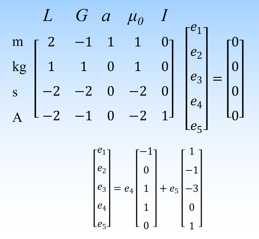
The next step in systematic dimensional analysis is to decompose the units for each physical quantity into fundamental units [8], e.g., 1T/m = m-1 kg s-2 A-1. The exponents e satisfy the homogeneous linear equation De=0, where D is called the dimensional matrix. Its n columns are labeled by the physical parameters, and its rows are labeled by the units (Fig. 1). In addition to the relevant basic SI units (m,kg,s and A), the fifth row in D represents the unit turns. This inclusion is motivated by the product N×I in units of amp-turns appearing commonly in transformer and coil design. Recall L scales as N2 and G scales linearly with N, allowing us to complete the bottom row of D (Fig. 1). For illustrative purposes, we also analyze the problem omitting turns as a unit, i.e., constructing the 4x5 dimensional matrix D’ (Fig.2).
In general, the number of linearly independent, non-zero solutions for e is given by n-rank(D), and is equal to the number of dimensionless products that can be formed. The solutions for e were determined by Gaussian elimination.
Results
The matrix D has rank=4, so there is only 5-4=1 distinct, non-zero solutions for e shown in Fig. 1. According to the Buckingham’s theorem [8], the resulting dimensionless quantity equals some constant, which dimensional analysis does not specify, yieldingL½ I μ0½ (G a5/2) -1 = const...….[1]
Squaring the expression in Eq.1, absorbing μ0 into the constant, and defining the gradient efficiency η≡GI -1 yields
L α (G2 I -2) a5 = η2a5….....……[2]
The quadratic dependence of inductance on gradient efficiency illustrates a fundamental tradeoff between maximal gradient amplitude and slew rate [1-2].
If instead “turns” is excluded as a row in the dimensional matrix D' (Fig. 2), then there are two distinct, non-zero solution to D'e=0 because rank(D')= 3. When there are two dimensionless parameters, Buckingham’s theorem implies they are related by an (unspecified) function [8]. This yields
a μ0/L = f[ LI (Ga3)-1 ]..............[3]
Typically the unspecified function f needs to be determined with further measurements or simulations. The scaling relation L α η2a5 can still be obtained from Eq. 3, but only with the choice f(x) = x-2 , which is equivalent to choosing e4 = ½ e5 in Fig 2. Without the physical insight of the dependence of L and G on turns, there is no a priori reason to make these choices.
Discussion and Conclusion
The analysis that includes the number of turns as unit is considerably more useful because the scaling relationship L α η2a5 emerges as the unique result. Unlike the analysis omitting turns and resulting in Eq. 3, no further measurements or simulations are required to obtain the unknown functional dependence in Eq.3. While turns is a dimensionless unit (i.e., not a length, mass, charge, etc.), this is not a concern. There are many other dimensionless units in commonly use, e.g., moles of a substance, or radians to measure angle, which is dimensionless since it is the ratio of two lengths.In conclusion, systematically applying dimensional analysis using linear algebraic tools and physically reasonable assumptions, we have derived the important scaling relation for gradient design: L α η2a5 . Use of turns in the dimensional matrix greatly simplifies the analysis.
Acknowledgements
This work was partially supported by research grant NIH U01 EB024450.References
1. Turner R. Gradient coil design: a review of methods. Magn Reson Imaging. 1993;11(7):903-20.
2. Hidalgo-Tobon SS. Theory of gradient coil design methods for magnetic resonance imaging. Concepts in Magnetic Resonance Part A, 2010; 36A(4) 223–242.
3. Lee SK, Mathieu JB, Graziani D, Piel J, Budesheim E, Fiveland E, Hardy CJ, Tan ET, Amm B, Foo TK, Bernstein MA, Huston J 3rd, Shu Y, Schenck JF. Peripheral nerve stimulation characteristics of an asymmetric head-only gradient coil compatible with a high-channel-count receiver array. Magn Reson Med. 2016 Dec;76(6):1939-1950.
4. In MH, Shu Y, Trzasko JD, Yarach U, Kang D, Gray EM, Huston J, Bernstein MA. Reducing PNS with minimal performance penalties via simple pulse sequence modifications on a high-performance compact 3T scanner. Phys Med Biol. 2020 Jul 31;65(15):15NT02.
5. Endt vom A, Kimmlingen R, Riegler J, Eberlein E, Schmitt F. A high-performance head gradient coil for 7T systems. Proceedings of the 14th Annual Meeting of the International Society of Magnetic Resonance in Medicine; 2006; p. 1370.
6. Foo TKF, Laskaris E, Vermilyea M, Xu M, Thompson P, Conte G, Van Epps C, Immer C, Lee SK, Tan ET, Graziani D, Mathieu JB, Hardy CJ, Schenck JF, Fiveland E, Stautner W, Ricci J, Piel J, Park K, Hua Y, Bai Y, Kagan A, Stanley D, Weavers PT, Gray E, Shu Y, Frick MA, Campeau NG, Trzasko J, Huston J 3rd, Bernstein MA. Lightweight, compact, and high-performance 3T MR system for imaging the brain and extremities. Magn Reson Med. 2018 Nov;80(5):2232-2245.
7. Foo TKF, Tan ET, Vermilyea ME, Hua Y, Fiveland EW, Piel JE, Park K, Ricci J, Thompson PS, Graziani D, Conte G, Kagan A, Bai Y, Vasil C, Tarasek M, Yeo DTB, Snell F, Lee D, Dean A, DeMarco JK, Shih RY, Hood MN, Chae H, Ho VB. Highly efficient head-only magnetic field insert gradient coil for achieving simultaneous high gradient amplitude and slew rate at 3.0T (MAGNUS) for brain microstructure imaging. Magn Reson Med. 2020 Jun;83(6):2356-2369.
8. Szirtes T. Applied dimensional analysis and modeling. McGraw-Hill 1997.
9. Bernstein MA, Friedman WA. Thinking about equations. Chapter 6, Introduction to dimensional analysis and scaling. Wiley 2009.
10. Pascone R, Vullo T, Cahill PT. Theoretical and experimental analysis of magnetic field gradients for MRI. 1993, available on IEEE Explore.
Figures