3099
MRI Hybrid Gradient Coil Equipped with a Programmable Z-Array and Conventional X- and Y- Elements1UMRAM, Bilkent University, Ankara, Turkey, 2Department of Electrical and Electronics Engineering, Bilkent University, Ankara, Turkey
Synopsis
A novel hybrid gradient coil consisting of two conventional actively shielded x/y gradient coils and a programmable active-shield z-gradient array coil is introduced and simulated. The proposed hybrid gradient coil can dynamically provide the required magnetic profile based on diverse applications in MRI. This is achieved by using a set of independent power amplifiers that feed the conventional coils and the array elements. To show the flexibility, three magnetic profiles are simulated: (a) a conventional profile; (b) a profile with twice z-gradient intensity and a shifted FOV; (c) a profile with quadruple z-gradient intensity when the active-shield is reverse fed.
Purpose
The conventional gradient coils and their active shields can be replaced by a set of programmable arrays. This makes the gradient sub-system to be highly customizable and offer a wider range of features in addition to the conventional functionalities.Method
Gradient arrays have been used for shimming and/or spatial encoding in different shapes, formats, and configurations1-11. Recently, our group introduced7-9 a programmable z-gradient array and its independently-controllable active-shield array12 as a new modality in MRI gradient coil design. The conventional coils and each of the array elements are fed by dedicated power amplifiers13 in a manner determined by the required magnetic profile within the FOV region. The array coils are self-balanced and finding a proper set of feeding waveforms leads to a constrained optimization problem that can be solved either externally or onboard. The target field method14 or a combinational scenario of analytical and numerical solutions may be used for best results. The programmability of the magnetic field profile for the z-gradient coil makes it possible to vary different performance parameters, including gradient intensity, FOV size, linearity error, and slew rate along the z-axis.Results
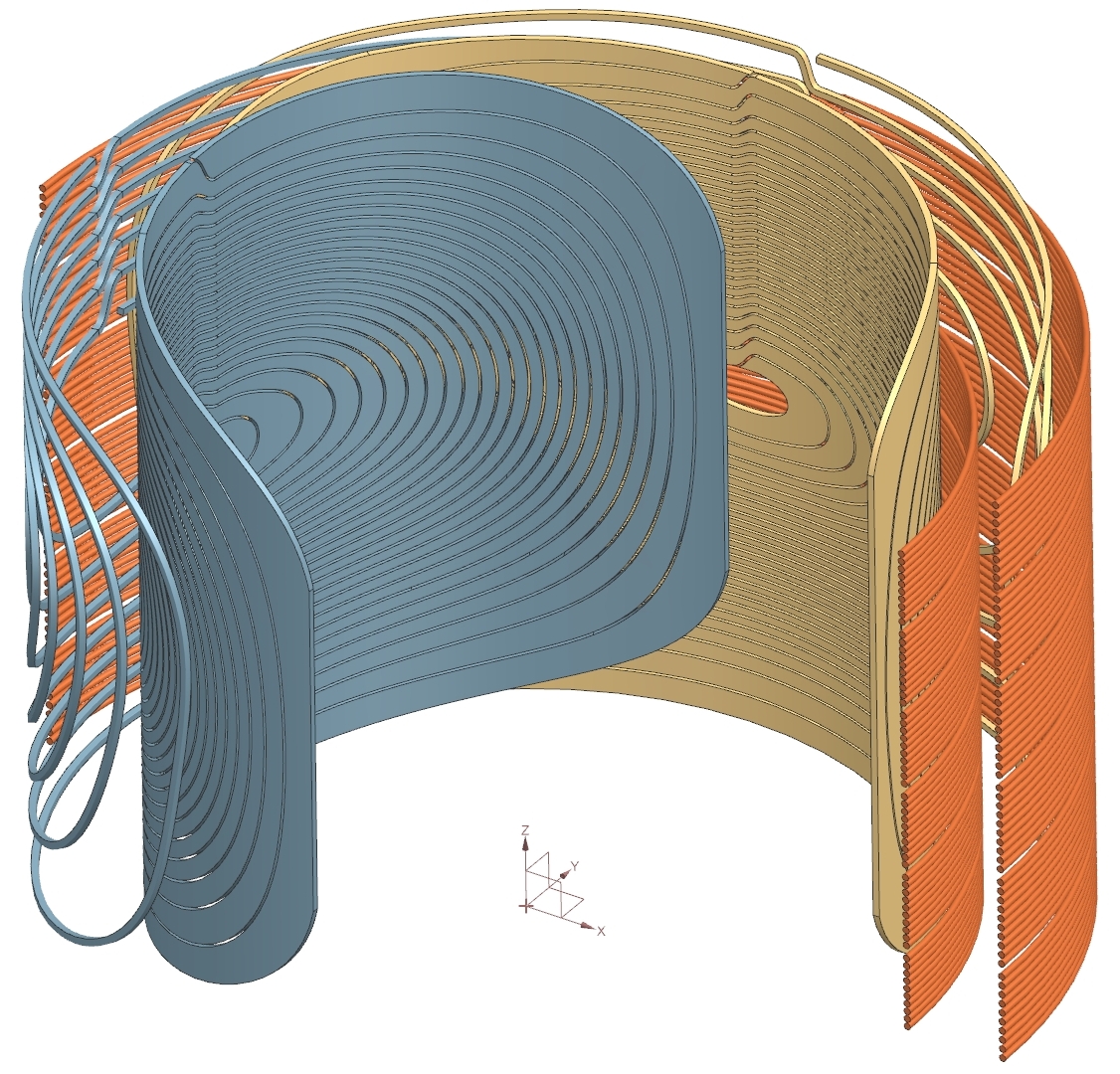
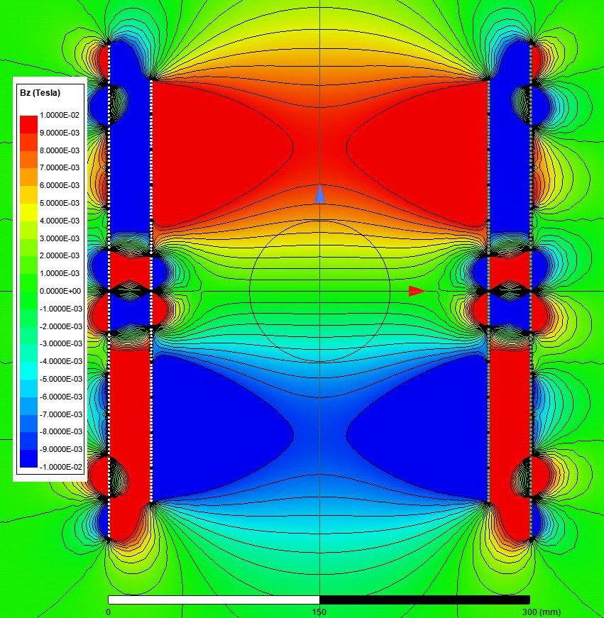
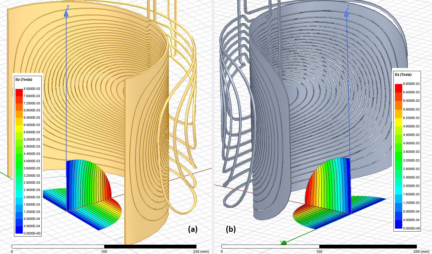
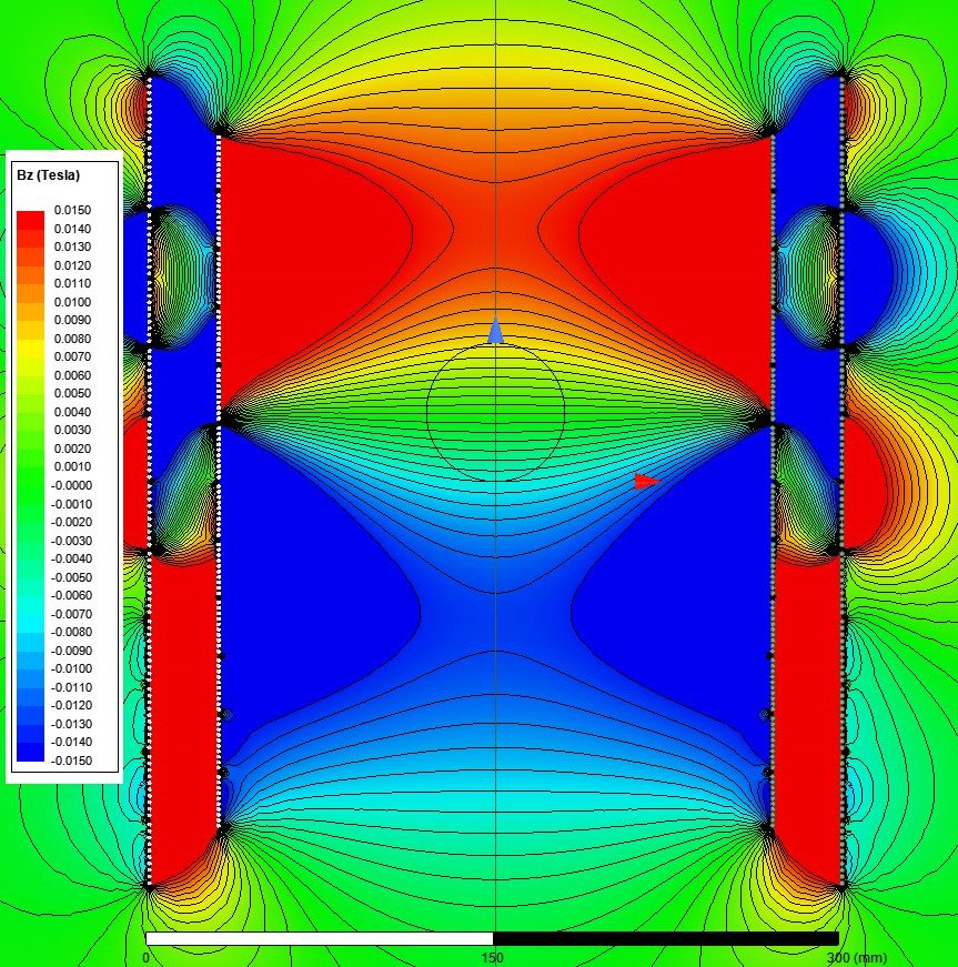
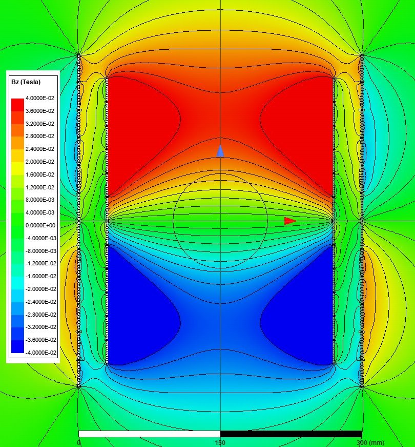
Figure 1 shows a small animal imagining gradient coil consisting of two conventional x- and y- gradient coils and a z-gradient array coil, where a quarter of each coil is shown for further clarity. Z-gradient array coil consists of 12 pairs of wire bundles, each with 10 copper wires of 2 mm diameter. The diameter/height of the main and the shield array coils are 24/30 and 30/35 cm, respectively. Copper sheets of 2 mm thickness and 40 cm height for the main coil and rectangular copper wires (2x2 mm2) are used for the shield coils. The diameter of the main/shield coil for the x- and y-gradient coils are 20/26 and 22/28 cm, respectively. For simulation, an aluminum cylindrical shell of 90 cm diameter is inserted to mimic the warm cryostat. For shield effectiveness assessment, we define the residual eddy current as the ratio of the Bz fields 20 us after to 20 us before the 100 us fall-time of trapezoidal feeding waveforms. The Bz field due to z-gradient array is shown in Fig. 2, where contour lines indicate 1 mT separations. The maximum current for all array elements is 100 A. The FOV diameter, linearity error, maximum gradient strength, and residual eddy current are 100 mm, 5.5%, 124 mT/m, and less than 0.0001%, respectively. Figure 3.a shows the y-gradient coil and the Bz field map inside the FOV region, where the contour lines indicate 0.4 mT separations. The FOV diameter, linearity error, and maximum gradient strength are 120 mm, 7.0%, and 128 mT/m, respectively. Similarly, Fig. 3.b shows the x-gradient coil and its field plot within the same FOV region. The gradient strength and linearity are 116 mT/m and 5%, respectively. The residual eddy currents are less than 0.023%. Both coils are fed by power amplifiers of maximum 100 A. Figure 4 shows the same gradient system with the second configuration for the z-gradient array profile. In this case, the FOV size is reduced to 60 mm and it is shifted up 30 mm along the z-axis. Z-gradient strength is doubled to be 250 mT/m within the shifted FOV region with less than 8.9% deviation from linearity. The contour lines indicate 1 mT separations. The linearity error and residual eddy current are 8.9% and 0.007%, respectively. Figure 5 shows the third configuration for the z-gradient array profile with a quadruple gradient strength of 506 mT/m and 4 mT separations. In this case, the FOV diameter, linearity error, and residual eddy current are 100 mm, 11%, and 0.004%, respectively. This is achieved by reverse feeding the shield array coil and utilizing the large enough gap between the cryostat and the coils. It should be emphasized that increasing the number of coils makes it possible to gain more degree of freedom and achieve a wider range of magnetic profiles within the FOV region by dynamically changing the amplitudes and waveforms of individual array elements12.Discussion
In the proposed hybrid structure, two conventional x- and y-gradient coils are equipped with a programmable active-shield z-gradient array to achieve a high degree of freedom for tuning the performance parameters of overall gradient assembly. Three cases are simulated to show its flexibility in changing the magnetic field profile on the fly. Another key feature of the proposed array system is its lower impedance of the array elements that makes it more suitable for higher switching frequencies.Conclusion
The benefit of a hybrid gradient coil is threefold: (a) magnetic field profiling is possible for a wide range of MRI applications due to the dynamic nature of the z-gradient coil; (b) it improves and speeds up the overall imaging speed since the impedance of the individual array elements are less than an equivalent conventional coil and its series-connected shield; (c) if shielding is not concerned, both of the main and shield array coils may be used constructively to achieve very high gradient strengths or slew rates. We expect that this realistic simulation study will lead to the construction of the gradient system in a near future.Acknowledgements
No acknowledgement found.References
1. Wintzheimer S, Driessle T, Ledwig M, et al. A 50-channel matrix gradient system: A feasibility study. Proc. of the ISMRM, Stockholm, Sweden. 2010:3937.
2. Juchem C, Rudrapatna SU, Nixon TW, de Graaf RA. Dynamic multi‐coil technique (DYNAMITE) shimming for echo‐planar imaging of the human brain at 7 Tesla. NeuroImage. 2015;105:462–472.
3. Juchem C, Green D, de Graaf RA. Multi-coil magnetic field modeling. Journal of Magnetic Resonance. 2013 Nov 1;236:95-104.
4. Juchem C, Nixon TW, McIntyre S, et al. Magnetic field modeling with a set of individual localized coils. Journal of Magnetic Resonance. 2010 Jun 1;204(2):281-9.
5. Jia F, Littin S, Layton KJ, et al. Design of a shielded coil element of a matrix gradient coil. Journal of Magnetic Resonance. 2017 Aug 1;281:217-28.
6. Littin S, Jia F, Layton KJ, et al. Development and implementation of an 84‐channel matrix gradient coil. Magnetic resonance in medicine. 2018 Feb;79(2):1181-91.
7. Ertan, K. , Taraghinia, S. , Sadeghi, A. and Atalar, E. (2018), A z‐gradient array for simultaneous multi‐slice excitation with a single‐band RF pulse. Magn. Reson. Med, 80: 400-412.
8. Ertan, K, Taraghinia, S, Atalar, E. Driving mutually coupled gradient array coils in magnetic resonance imaging. Magn Reson Med. 2019; 82: 1187– 1198.
9. Ertan, K., Taraghinia S, Sarıtas EU, Atalar E. Local optimization of diffusion encoding gradients using a z-gradient array for echo time reduction in DWI. In Proceedings of the 26th Annual Meeting of ISMRM, Paris, France, 2018. Abstract# 3194.
10. Kroboth S, Layton KJ, Jia F, Littin S, Yu H, Hennig J, Zaitsev M. Optimization of coil element configurations for a matrix gradient coil. IEEE Trans Med Imaging. 2018; 37:284–292.
11. Smith E, Freschi F, Repetto M, Crozier S. The coil array method for creating a dynamic imaging volume. Magn Reson Med. 2017; 78: 784– 793.
12. Takrimi, M. and Atalar, E. A Programmable Set of Z-Gradient Array and Active-Shield Array for Magnetic Resonance Imaging. ISMRM, Virtual, 2020.
13. Babaloo, R., Taraghinia, S., Acikel, V., Takrimi, M. and Atalar, E. Digital Feedback Design for Mutual Coupling Compensation in Gradient Array System. ISMRM, Virtual, 2020.
14. R. Turner, “A target field approach to optimal coil design,” Journal of physics D: Applied physics, vol. 19, no. 8, p. L147, 1986.
Figures